This blog shares the latest version of our synthetic-data pipeline for generating better training data with Blender. We render a synthetic view of the textile on a table from different camera angles, then pass each render through a generative model to produce a photorealistic image, with variance such as crumpled or folded textures introduced through the prompt. This adds disturbances that Blender’s simulation alone can’t produce. A vision LLM judge then compares the generated image against the original synthetic render to verify that orientation and other similarity conditions still match.
This solves a real problem: without a reference image, camera-angle variance has to be described entirely through the prompt, which is imprecise. A synthetic render gives the model something concrete to match, so the angle stays under control. This synthetic data is used for pre-training, with a much smaller sample of real data reserved for fine-tuning.
Setting the Blender scene: core concepts
Asset sourcing
The T-shirt mesh is a downloaded 3D asset (glTF format, from Sketchfab) and the table is a separate downloaded asset (FBX format), rather than being modeled from scratch. glTF was preferred for the T-shirt since it’s a lightweight, web-compatible format that keeps texture references bundled.
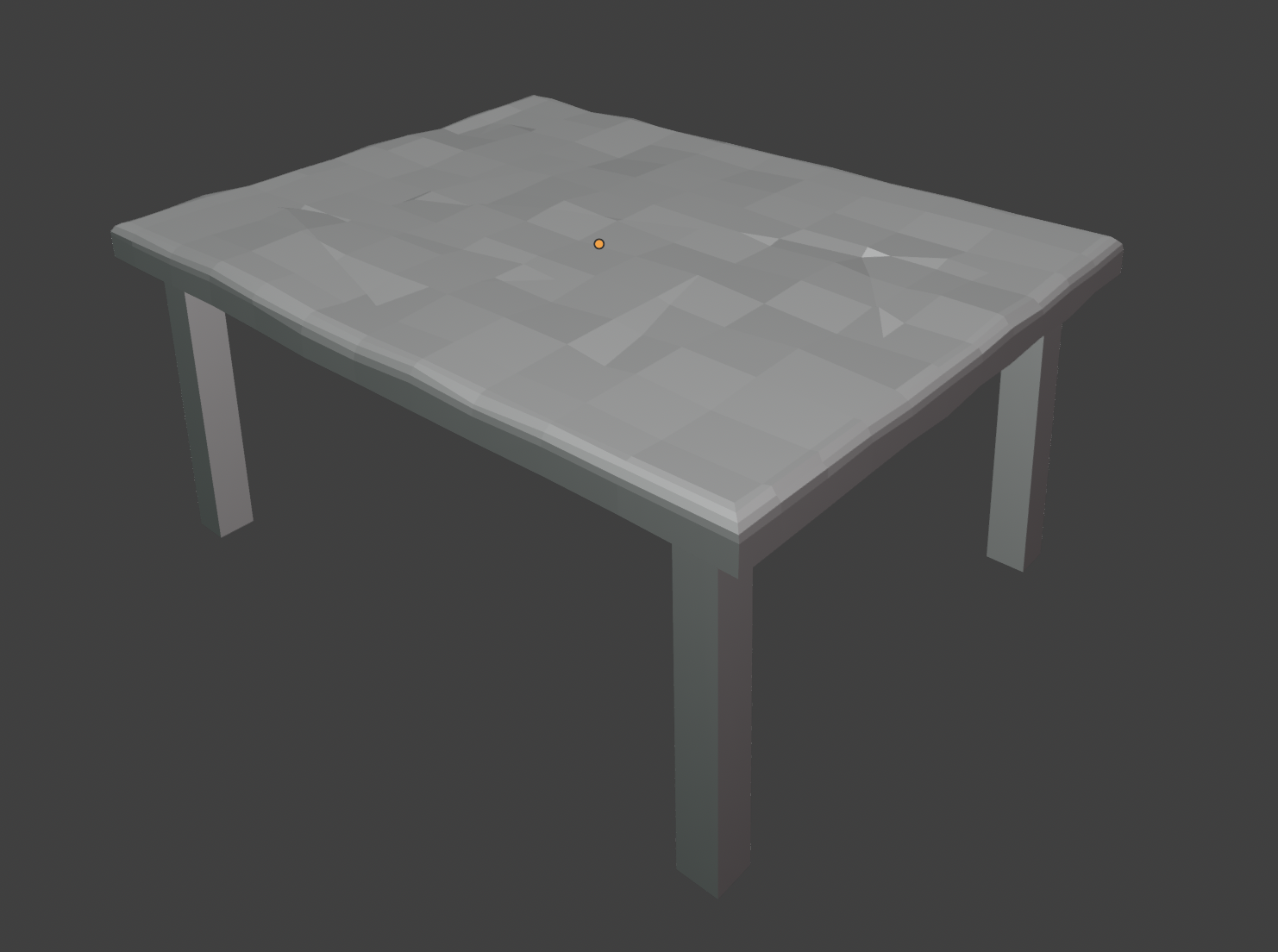
The table asset imported into the scene.
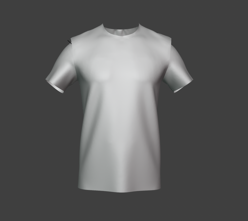
The T-shirt asset imported into the scene.
Scene composition
The table is placed first, with the T-shirt on top. A small amount of overlap between the two is fine since the training data only needs “textile placed on a table,” not pixel-perfect contact. The scene itself stays static; all the variation needed for training comes from randomizing the T-shirt’s orientation and the camera’s viewpoint, not from animating scene properties.
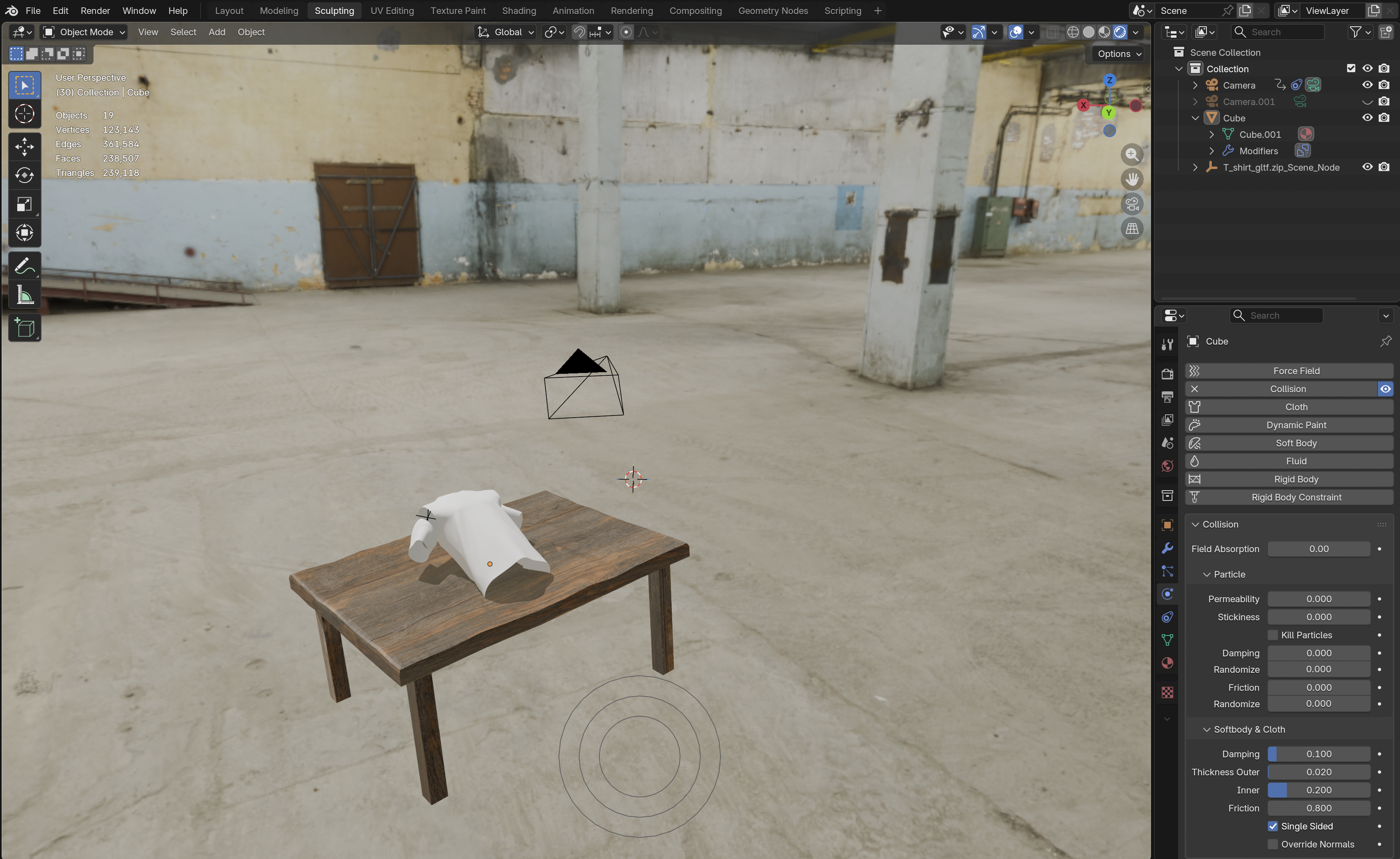
The full Blender setup, showing the table and T-shirt meshes, the cloth physics settings, and the camera in the outliner.
Camera perspective rationale
The camera setup mirrors real-world deployment, where the recognition system captures the textile from a top-down angle, either a fixed overhead camera or one mounted on a robotic arm. To match those conditions, the synthetic camera angles are also sampled around a top-down viewpoint.
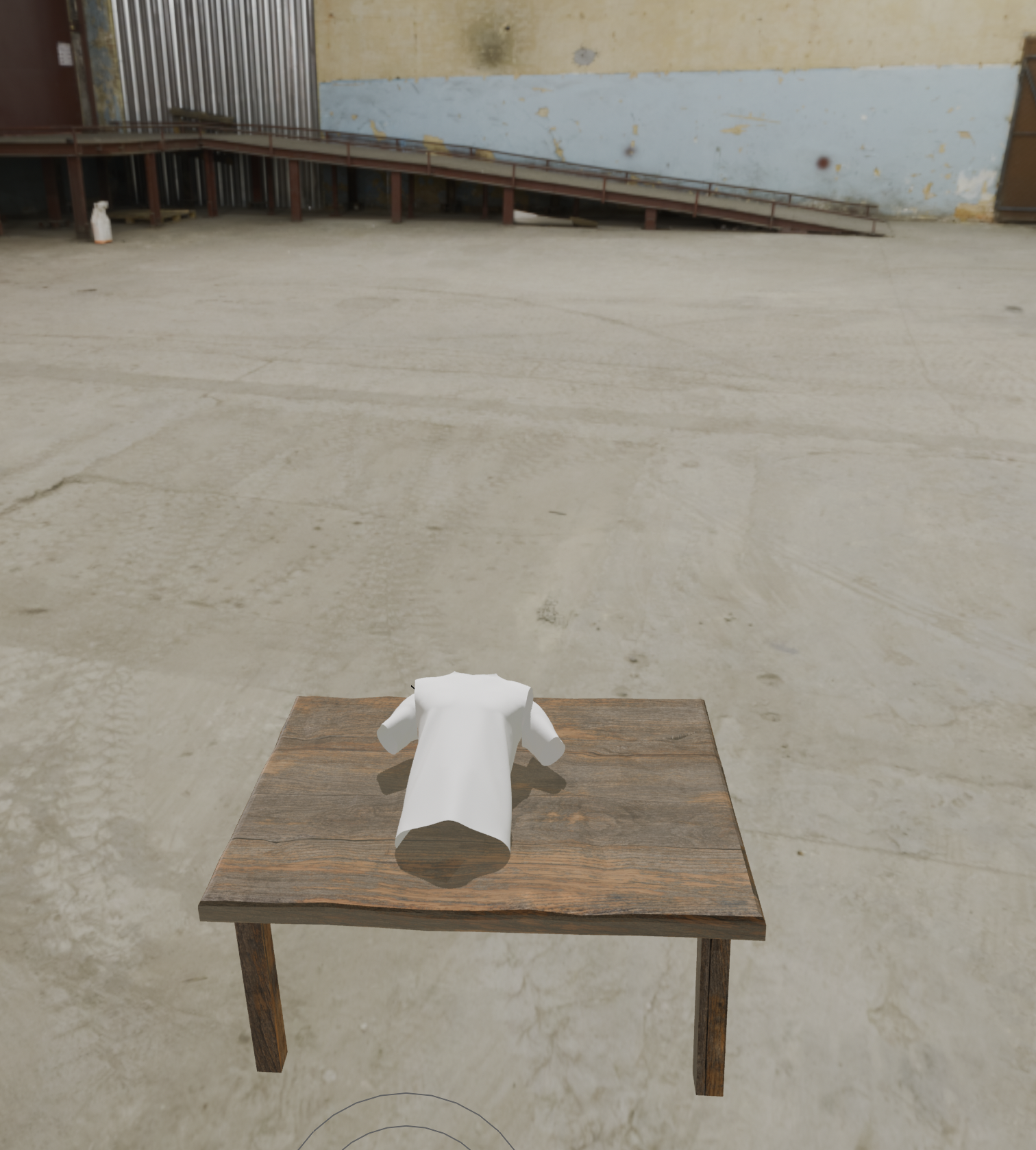
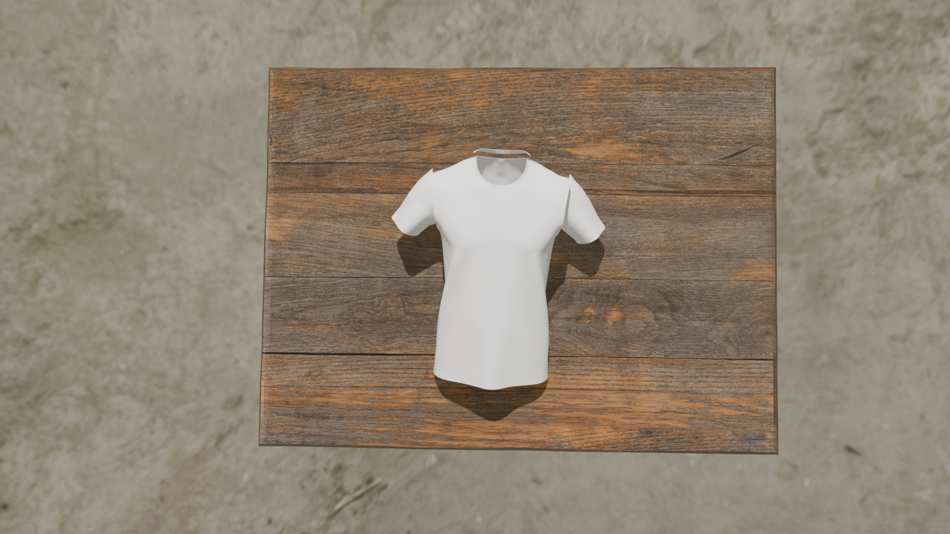
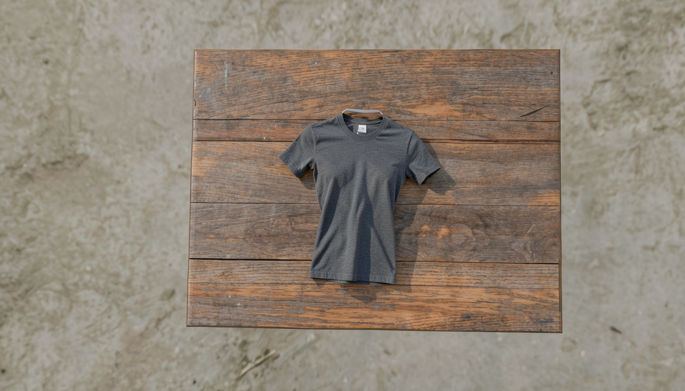
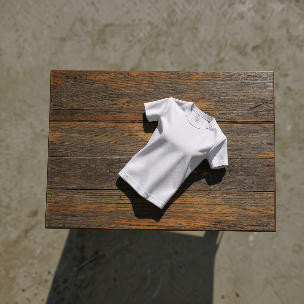
A sample render from the camera’s own viewpoint, showing the T-shirt on the table against the HDRI warehouse backdrop.
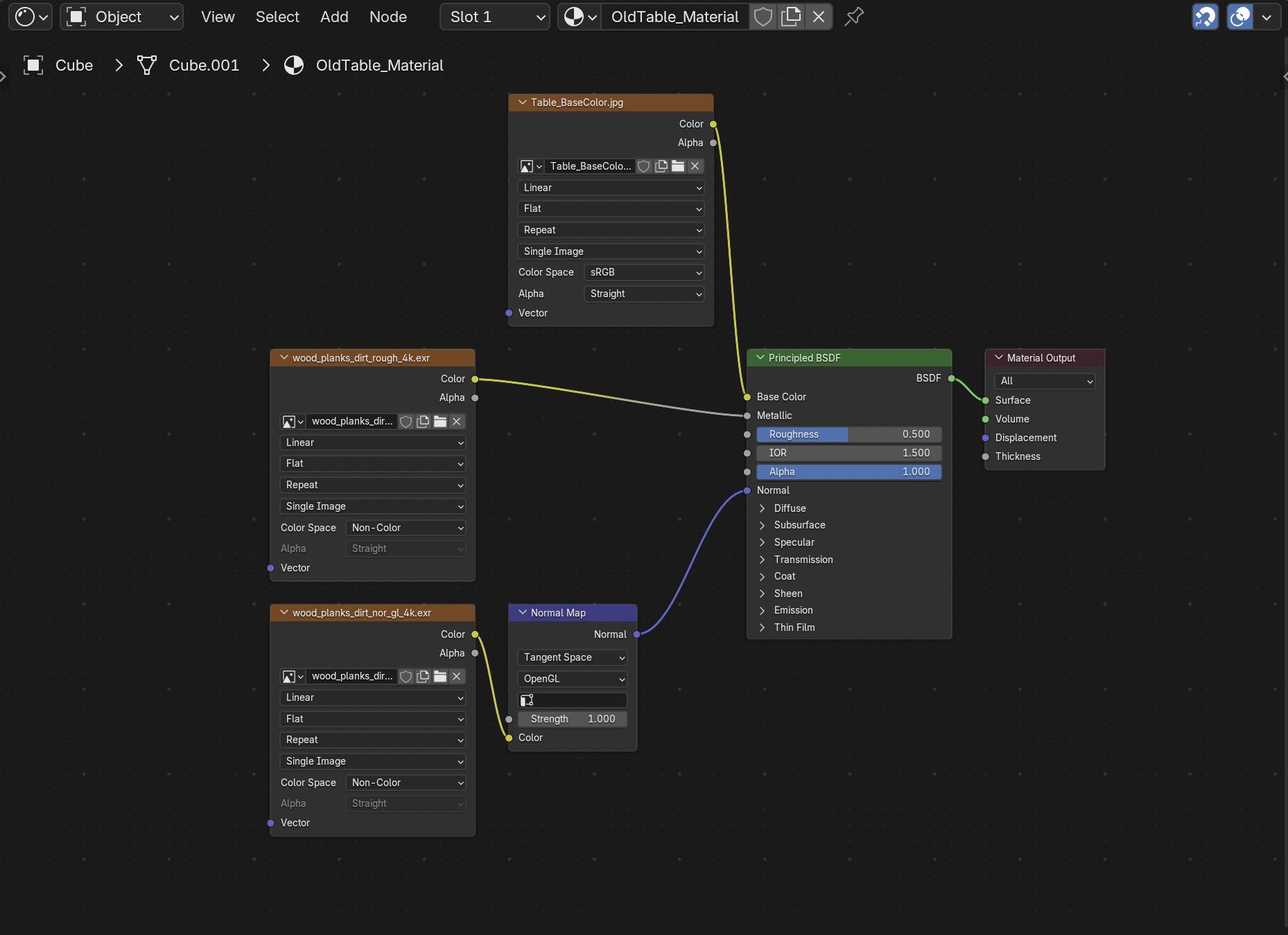
Material representation
A freshly imported 3D model has no shading by default; it renders as flat gray until a material is authored. Materials in Blender are built as a PBR node graph feeding a Principled BSDF shader. Three maps matter for textile specifically:
- Base Color: the surface color, in sRGB space.
- Roughness: matte vs. glossy, in Non-Color space.
- Normal map: fine surface detail like weave and folds, also Non-Color, converted into a usable normal vector before it reaches the shader.
Getting the color space right per map is the concept that matters: mixing it up (e.g., leaving a roughness map in sRGB) silently produces incorrect shading.
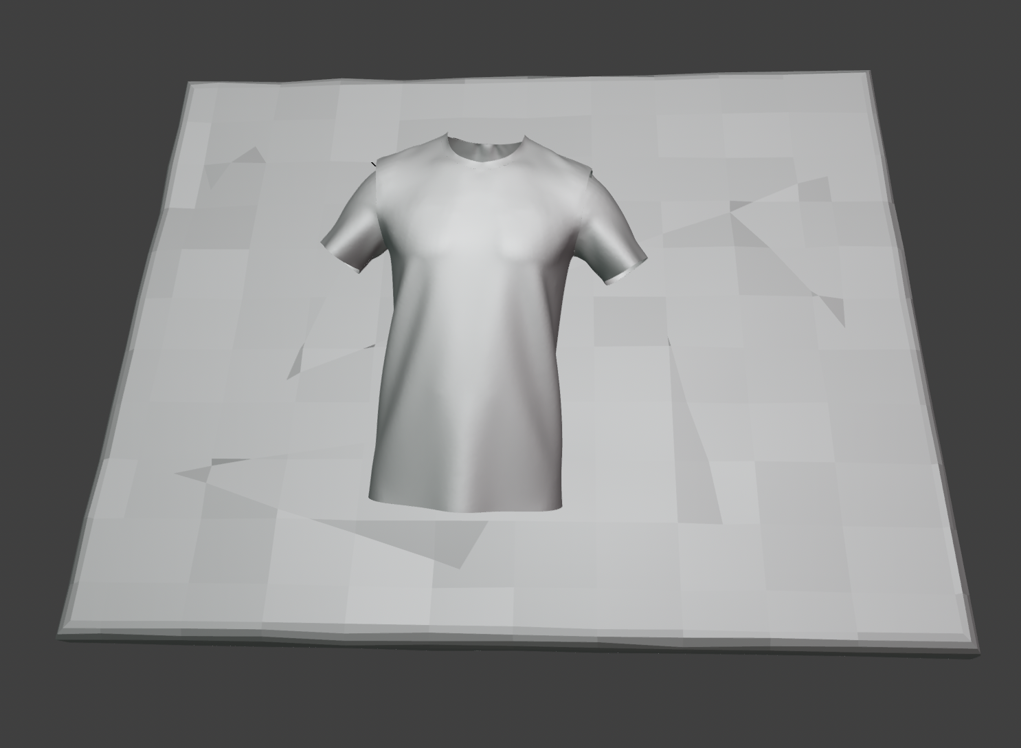
The T-shirt mesh with no material applied yet, rendered as flat gray.
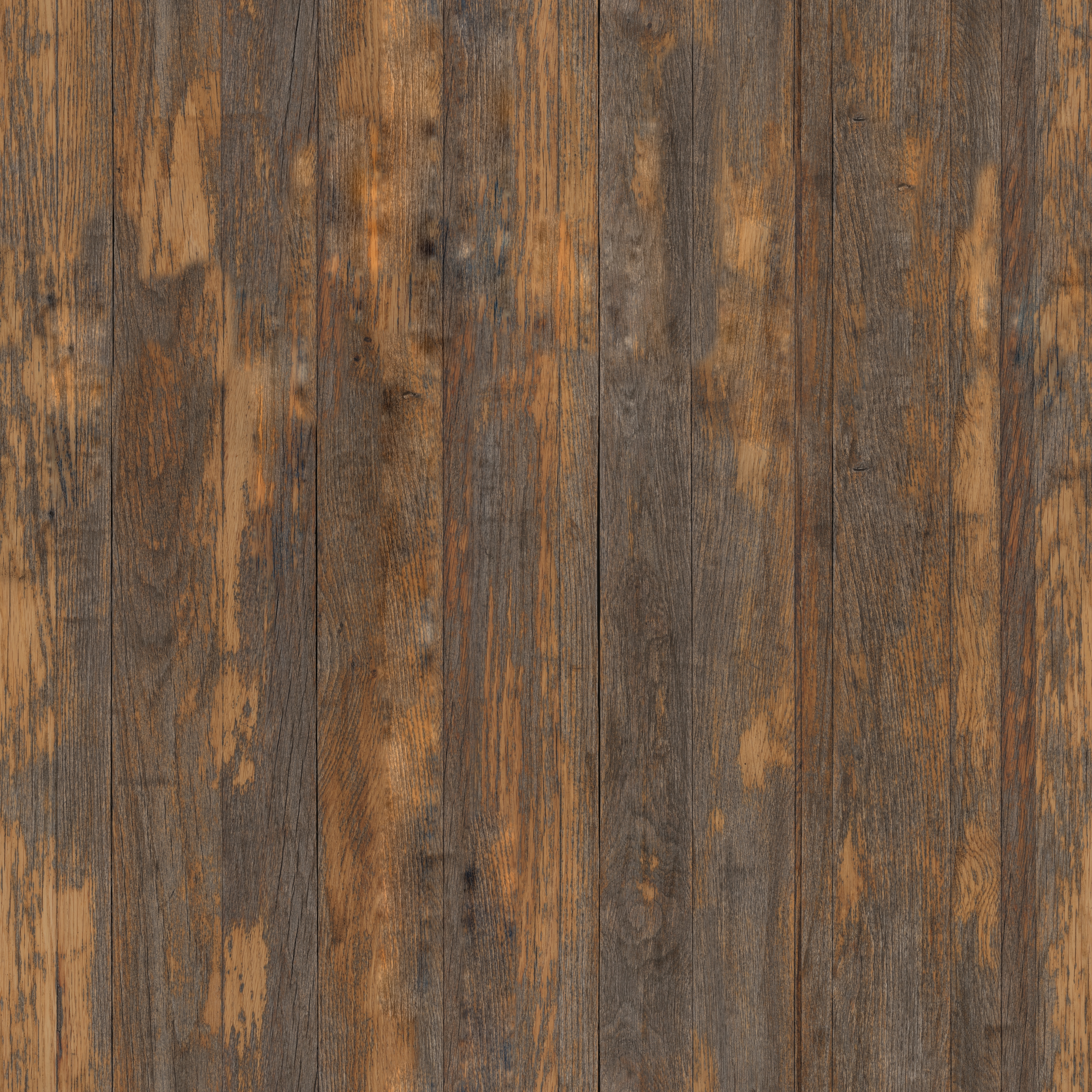
The table’s base color (albedo) texture used for its material.
The table rendered with its material and shading applied.
Setting up the shading nodes for the table’s material.
Lighting concept
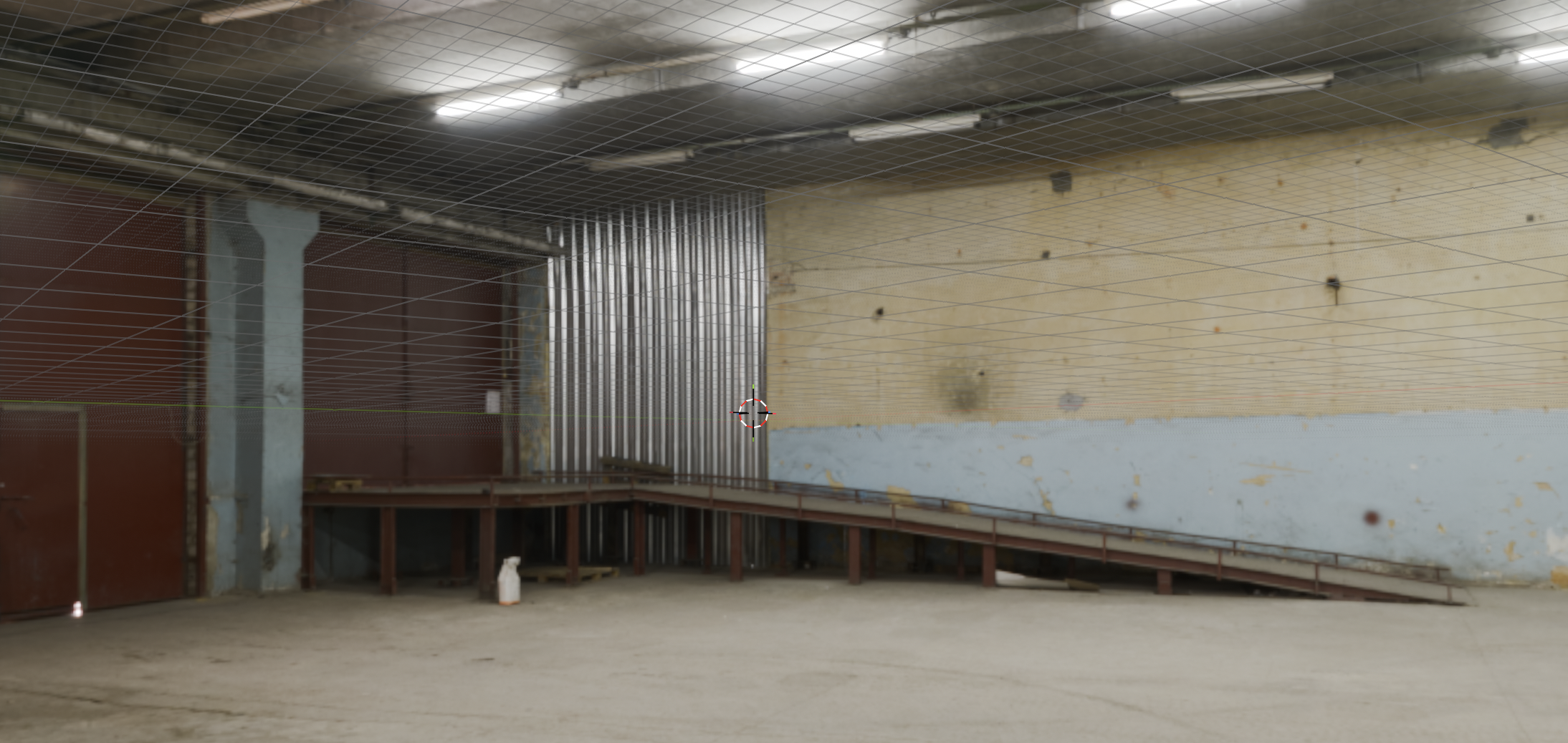
Lighting is treated as a variable, not a constant, since the recognition model needs to generalize across real-world conditions like harsh factory light, dim shadows, and overcast daylight. Instead of hand-placing lights, we use an HDRI, a 360° photo of a real environment, as world lighting; it supplies both ambient light and realistic reflections in one step. We use free warehouse HDRIs (e.g., from Poly Haven) to match the target deployment setting: a textile sorting facility.
The HDRI environment map providing the scene’s lighting and reflections.
Multi-view capture strategy
Instead of a single fixed shot, each iteration randomizes the T-shirt’s rotation and orbits the camera within a positional range above the table, generating many viewpoints per simulated drape.
A Track-To constraint keeps the camera aimed at the table’s center no matter where it’s randomly placed, so every render stays framed on the subject instead of drifting into empty background. This also fixes the earlier bug where a bad camera placement clipped the textile out of frame.
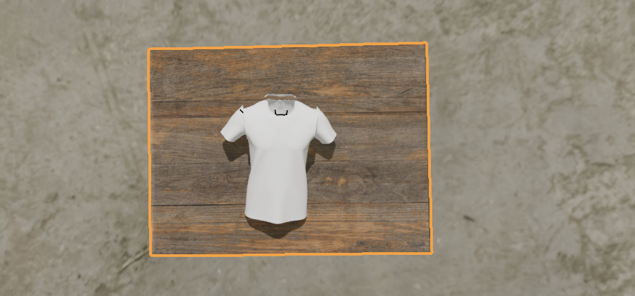
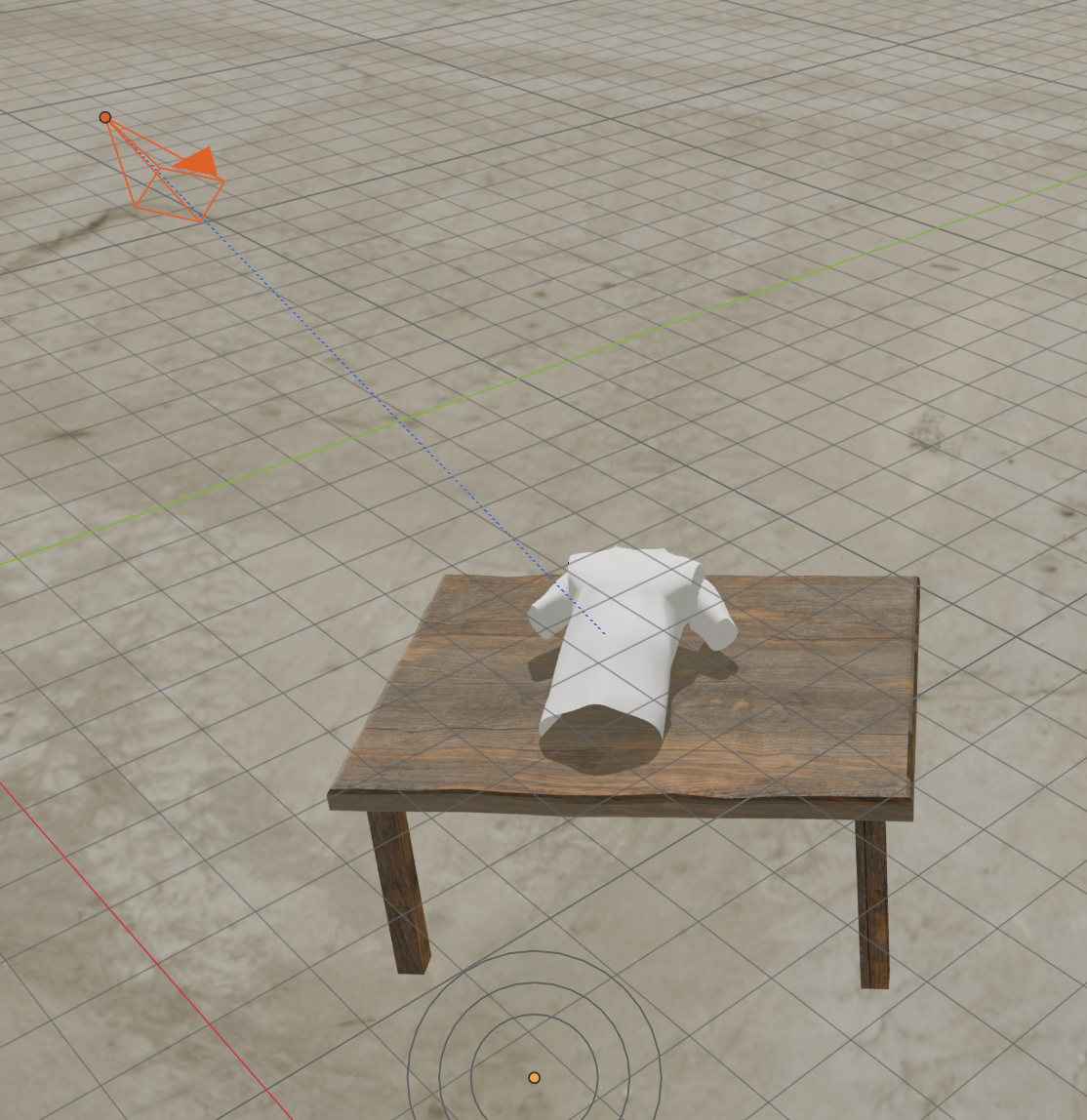
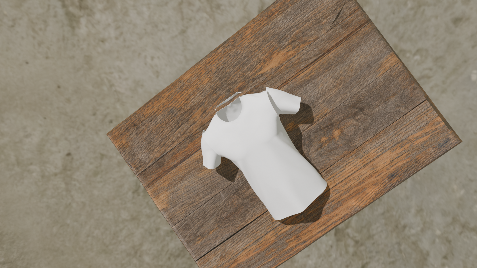
The first sampled camera angle looking down at the table.
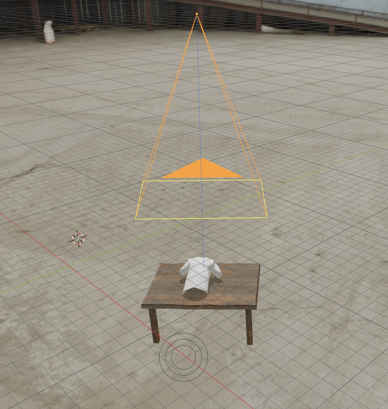
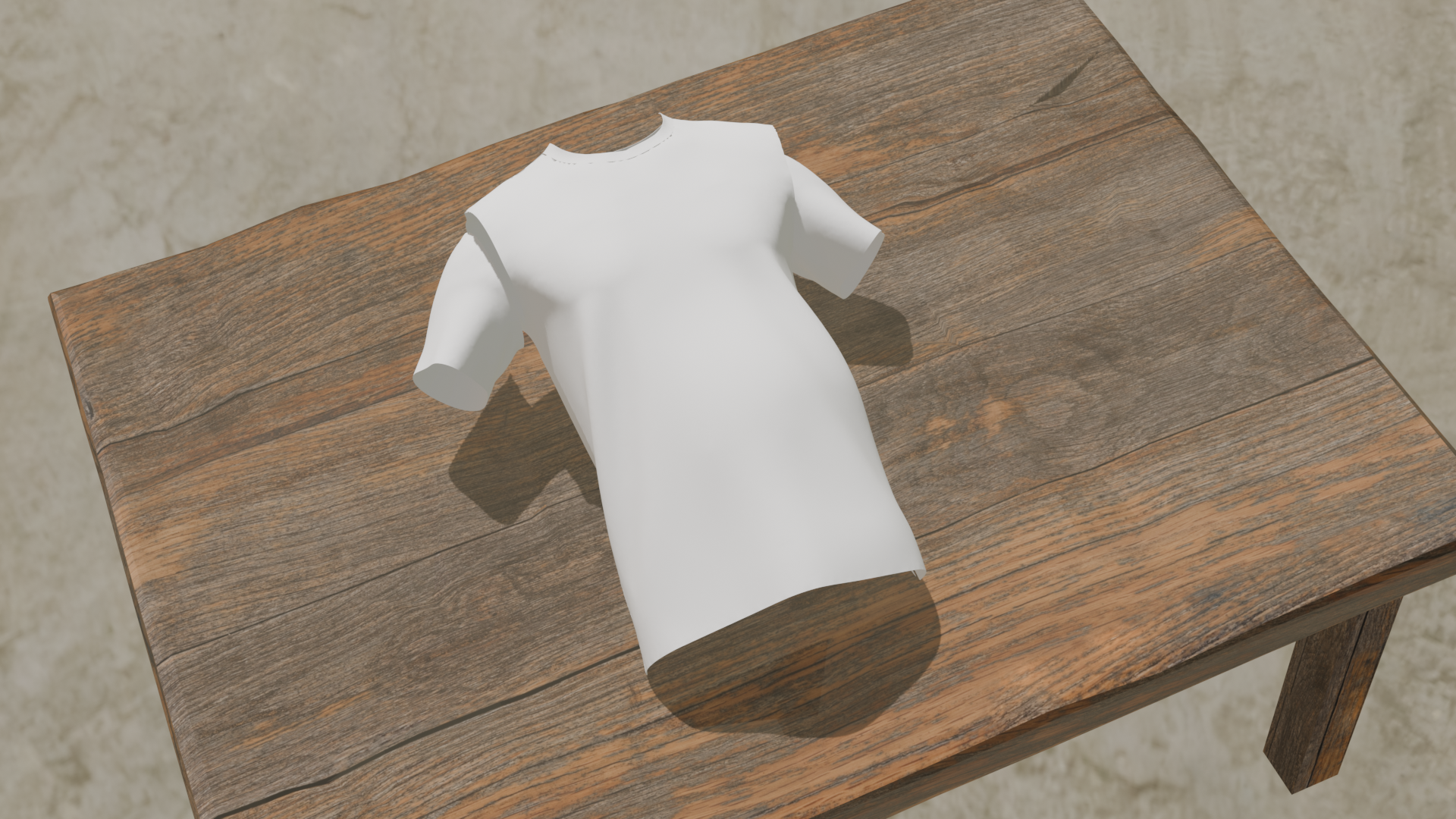
The second sampled camera angle looking down at the table.
Rendering as the final step
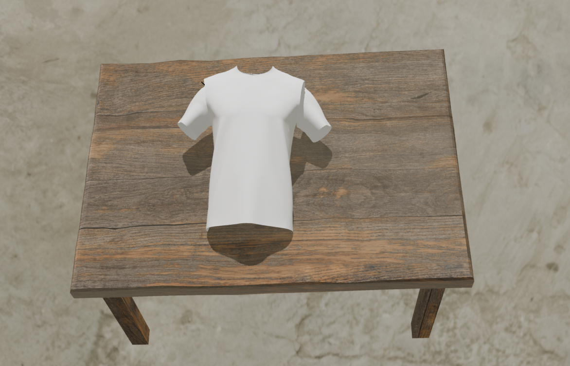
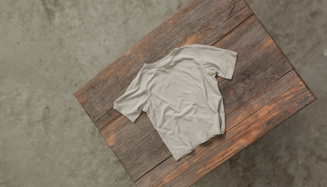
Once mesh, material, lighting, and camera are set for a given iteration, rendering converts that 3D scene state into a single 2D image, which becomes one training sample. Repeating this loop with fresh randomization each time produces the dataset of varied synthetic renders that later get passed to the generative model.
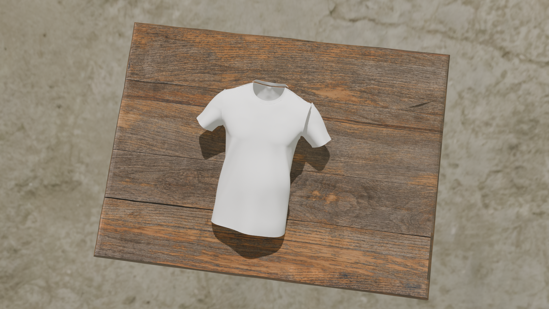
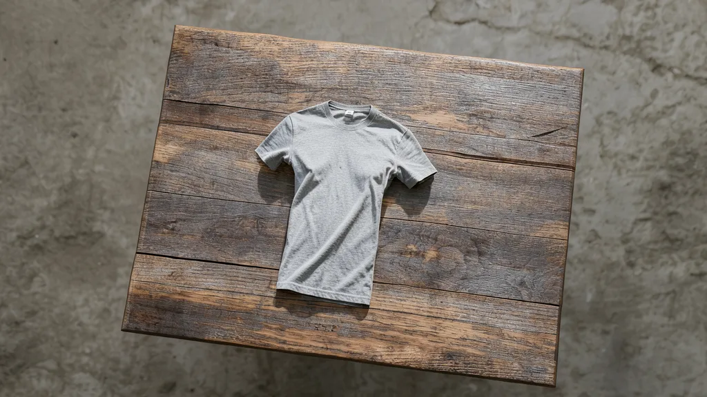
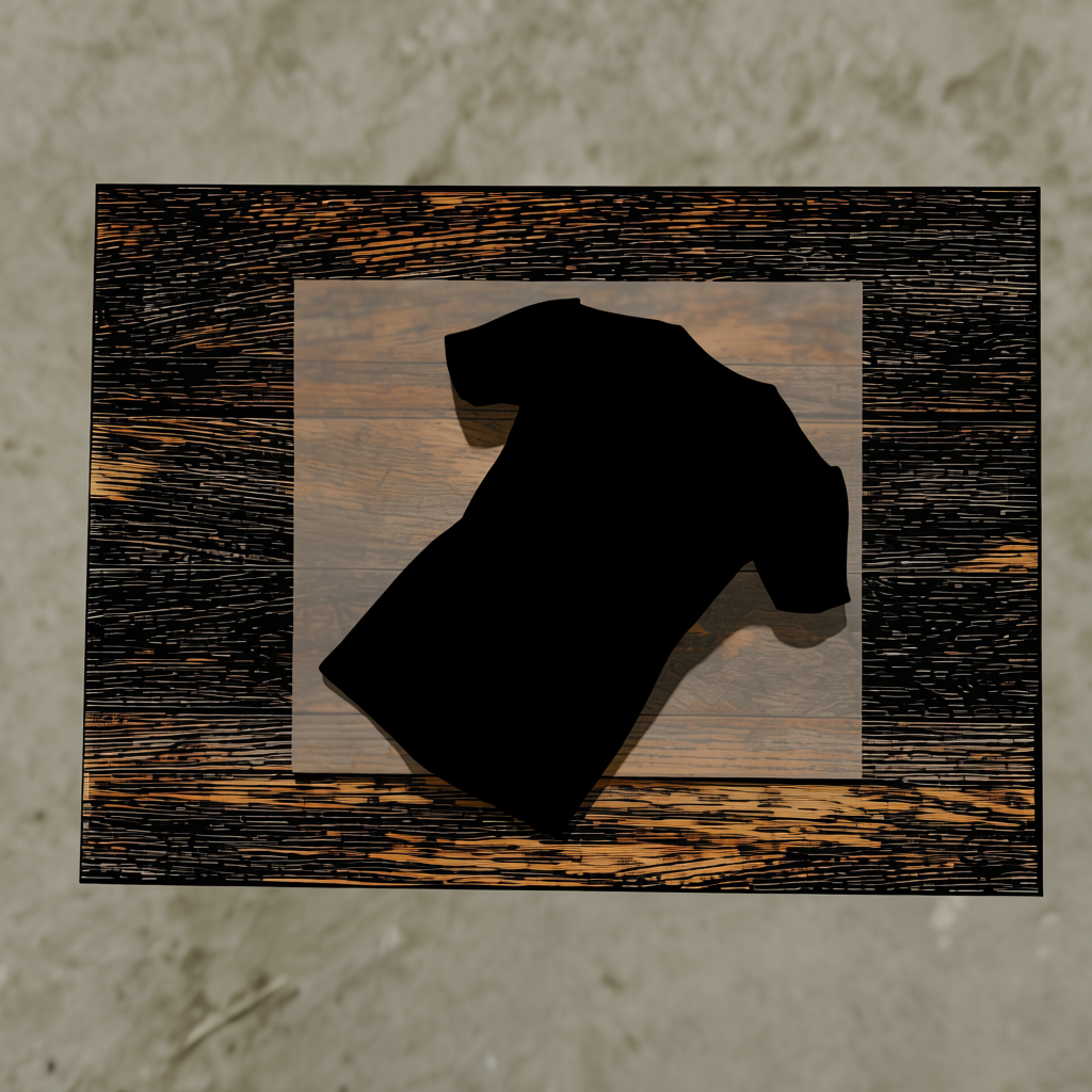
Different synthetic renders of the T-shirt on the table, captured from varying camera angles.
Generating photorealistic images
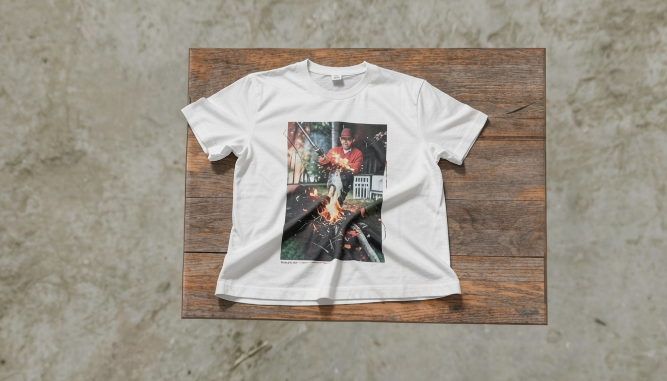
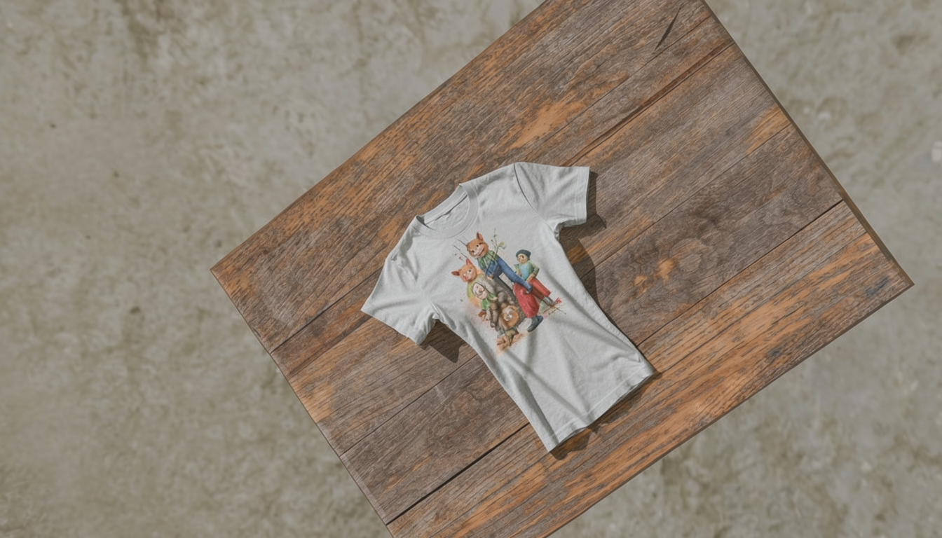
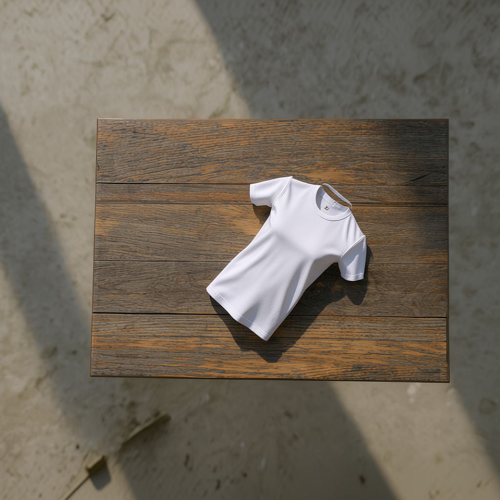
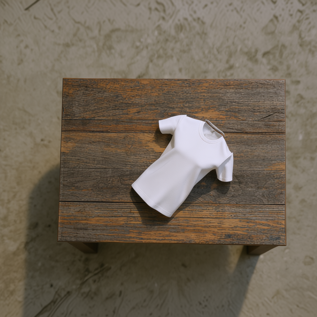
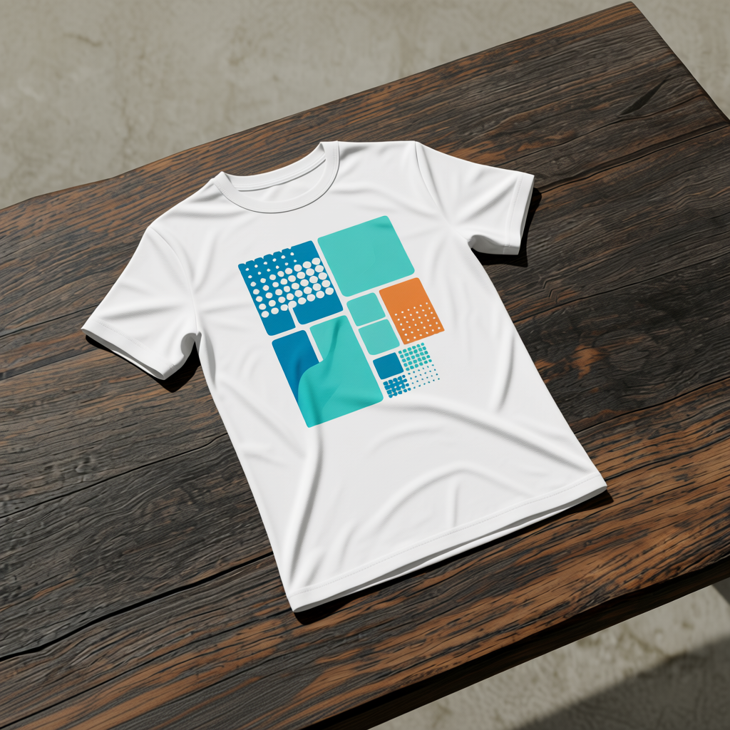
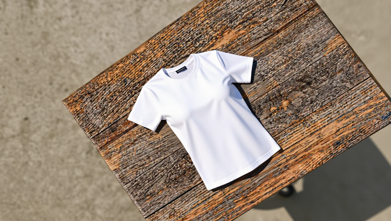
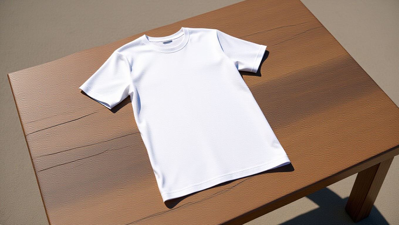
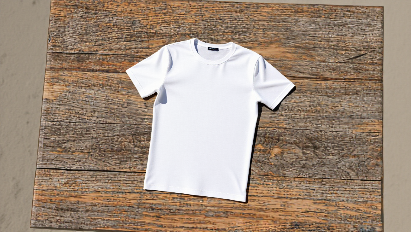
Each synthetic render is then passed through FLUX.2, Qwen to produce a photorealistic generated image.
| Synthetic render | FLUX.2 generated |
|---|---|
|
|
|
|
|
.png)
|
|
.webp)
|
| Synthetic render | Qwen generated |
|---|---|
 |
|
|
.png)
|
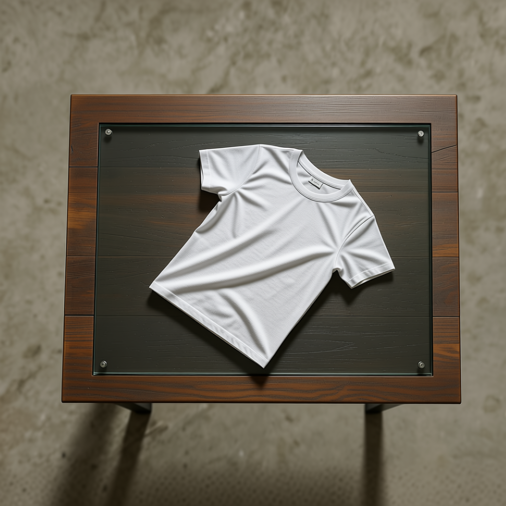
| Synthetic render | flux_edit generated |
|---|---|
|
|
|
|
|
|
Both the distilled and base variants of the model were tried, and they come with a clear time-complexity trade-off: the distilled variant (4 steps) takes 10–20s per image, while the base variant (50 steps) takes approximately 2 minutes, even on an optimized inference engine.
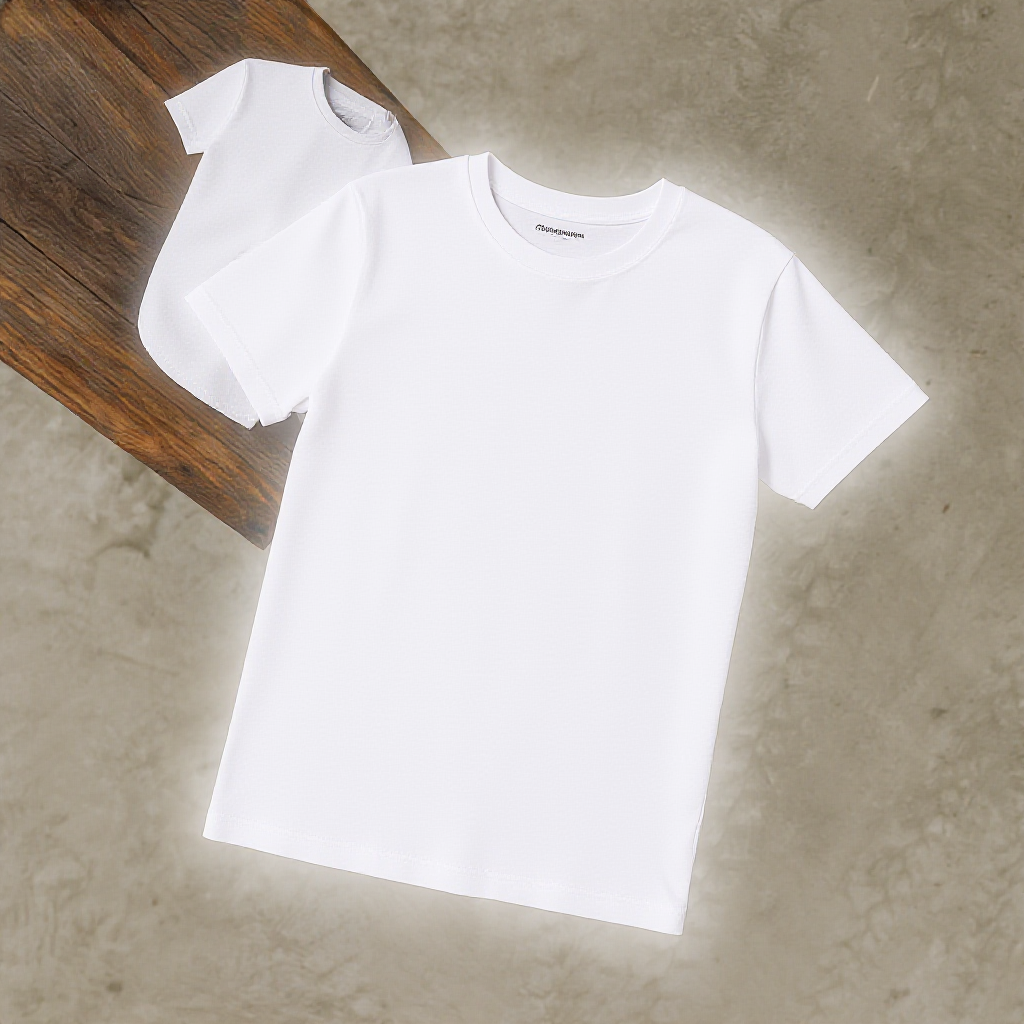
Failed generations
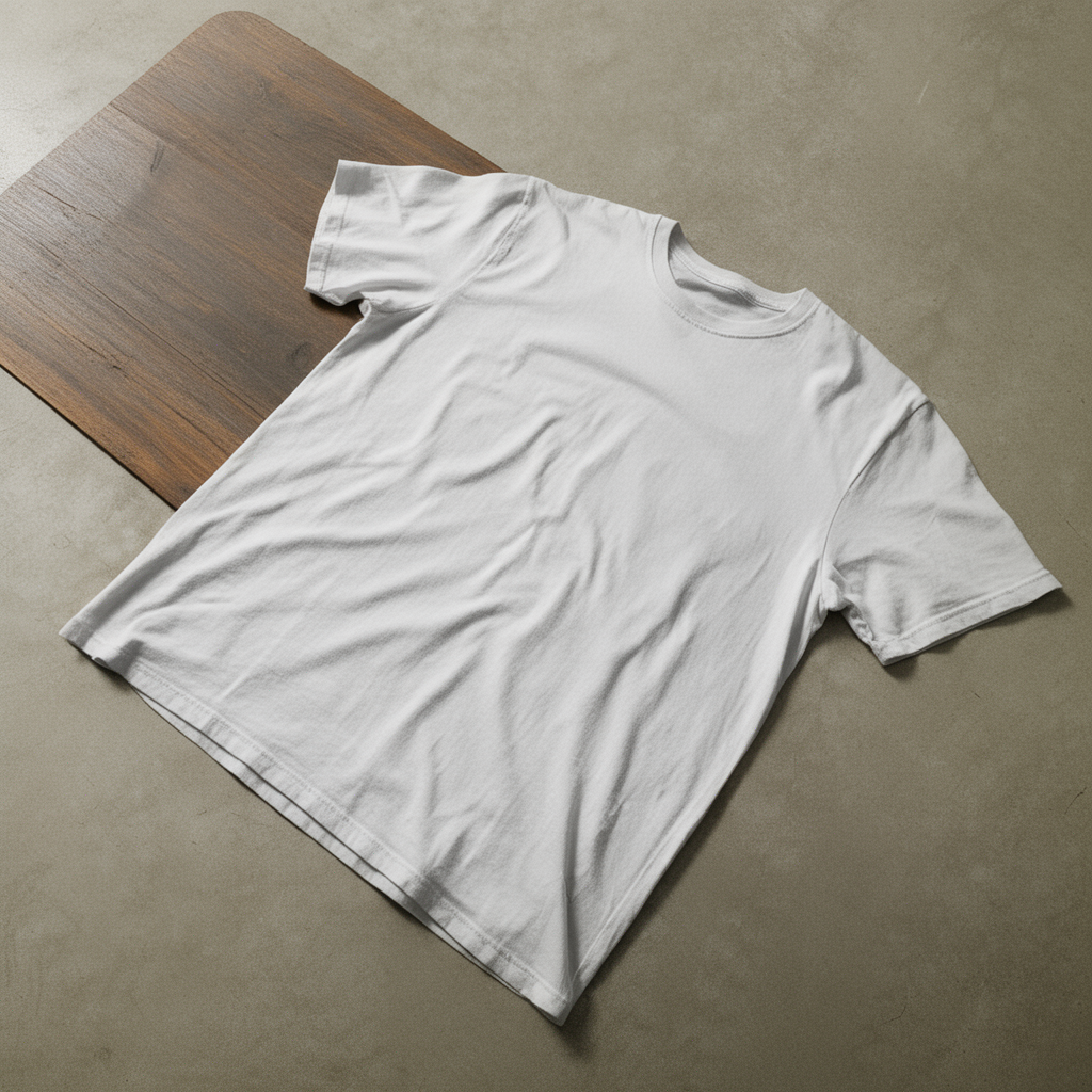
- Collapsed table: the table is collapsed, leaving the T-shirt floating with almost no surface context.
- Enlightened T-shirt: a ghosted, duplicated T-shirt artifact in the upper-left of the generated image.
Evaluation
The simplest evaluation uses a vision LLM judge: it compares the synthetic render against the generated image and returns a similarity score, covering orientation, T-shirt placement, and relative scale.
Judging modes we use
| Mode | Image editing | T2I generation |
|---|---|---|
| Prompt tuning | Edit + evaluate, then refine the prompt | Generate + evaluate, then refine the prompt |
| Pointwise | Score one edit against its source + instruction | Score one generation against its prompt |
| Pairwise | Compare two edits, pick the better one | Compare two generations, pick the better one |
Evaluation metrics
- How many of the images match the similarity – “Similarity” here is semantic, not pixel-level: the FLUX.2 pass is expected to change texture, color, and photorealistic style, since that’s the whole point of the transformation. What must be preserved:
| Constraint | What it checks |
|---|---|
| Orientation | The T-shirt’s facing matches the synthetic reference. |
| Placement | The T-shirt stays fully on the table surface, with no floating or clipping outside the table bounds. |
| Scale | The table reads as proportionately larger than the T-shirt, not visually shrunk or dominating. |
| Integrity | Exactly one T-shirt, no duplicated or ghosted garments. |
| Pose | The fold state is still recognizable as the same pose as the synthetic render. |
A generated image “matches” only if the vision LLM judge scores it as satisfying all of these constraints, not just some of them.
- What are the improvements that could be done – This splits into two levels:
- Image generation quality – better prompt conditioning to preserve scene geometry (table boundaries, occlusion regions), and choosing the base (50-step) model over the distilled (4-step) one when fidelity matters more than generation speed.
- Pipeline level – replacing a purely vision-LLM-judge similarity score with the physics-informed metric noted below, and feeding failure cases back into prompt iteration rather than treating each generation as a one-shot attempt.
In practice, we score each generated image using a weighted combination of the vision LLM judge and classical image-processing checks, and use that combined score to validate the image before it’s admitted into the pre-training pipeline.
Insights from our data
- Occlusion regions are where the model struggles most: samples with occluded T-shirt or table regions consistently showed generation issues.
- A physics-informed metric would catch these failure modes more reliably than the current vision LLM judge alone.
- Getting to the best generated image took several rounds of prompt iteration rather than a single pass.
Conclusion
Pairing Blender’s synthetic renders with FLUX.2/Qwen/flux_edit generation gives us a controllable way to inject real-world variance such as lighting and disturbances that the simulation alone can’t produce, while the vision LLM judge keeps generated images anchored to the original orientation, placement, and scale. The main open gap is occlusion handling, which is where we’re focusing next, alongside folding in a physics-informed metric to complement the LLM judge.