Karthik Tech Blogs
Visualize feature maps
In this article, I will visualize the feature maps in a neural network. Since the focus of this article is to visualize the feature maps, I am using a tutorial neural network training script from PyTorch official website. This tutorial uses Transfer learning with Resnet50 architecture. The complete tutorial script can be found here.
Visualizing the feature map gives a better model interpretable capability. These feature maps can used to decide upon the number of hidden layers, type of convolution, kernel size and other hyperparameters. Since neural networks are deployed in production application such as autonomous cars, there must be a systematic approach to set the hyperparameters instead of grid search or random walk. Grid search or random walk increases the computation cost by experimenting with different values, which fails to explain the intent behind choosing a specific values.
I will use PyTorch hooks to extract intermediate layer outputs. Hooks can be called during forward or backward pass. You can find about hooks here. I have used forward hook, since we are visualizing the intermediate forward feature maps. In case, if we must visualize the gradients, we can use the backward hooks. Hooks also provides an advantage to modify the backward gradients.
Let’s get started now !!!
from __future__ import print_function, division

import torch
import torch.nn as nn
import torch.optim as optim
from torch.optim import lr_scheduler
import numpy as np
import torchvision
from torchvision import datasets, models, transforms
import matplotlib.pyplot as plt
import time
import os
import copy


BATCH_SIZE = 100


# Data augmentation and normalization for training
# Just normalization for validation
data_transforms = {
    'train': transforms.Compose([
        transforms.RandomResizedCrop(224),
        transforms.RandomHorizontalFlip(),
        transforms.ToTensor(),
        transforms.Normalize([0.485, 0.456, 0.406], [0.229, 0.224, 0.225])
    ]),
    'val': transforms.Compose([
        transforms.Resize(256),
        transforms.CenterCrop(224),
        transforms.ToTensor(),
        transforms.Normalize([0.485, 0.456, 0.406], [0.229, 0.224, 0.225])
    ]),
}


data_dir = '/content/hymenoptera_data'
image_datasets = {x: datasets.ImageFolder(os.path.join(data_dir, x),
                                          data_transforms[x])
                  for x in ['train', 'val']}
dataloaders = {x: torch.utils.data.DataLoader(image_datasets[x], batch_size=BATCH_SIZE,
                                             shuffle=True, num_workers=4)
              for x in ['train', 'val']}
dataset_sizes = {x: len(image_datasets[x]) for x in ['train', 'val']}
class_names = image_datasets['train'].classes

device = torch.device("cuda:0" if torch.cuda.is_available() else "cpu")
Defining a class for forward hooks. register_forward_hook calls the function save_activation with parameters name and epoch.
from functools import partial

class HooksExecution(nn.Module):
    def __init__(self, model: nn.Module, epoch):
        super().__init__()
        self.model = model

        # Register a hook for each layer
        for name, layer in self.model.named_children():

            # looping through each layer
            layer.__name__ = name
            layer.register_forward_hook(partial(save_activation, name, epoch))


    def forward(self, x: Tensor) -> Tensor:
        return self.model(x)
I am using an universal unique identifier for activations dictionary keys to avoid overwriting. This can be optimized.
activations = {}

def save_activation(name, epoch, batch, mod, inp, out):

  random_gen = str(uuid.uuid4())[-5:]
  activations[f"{epoch}_{batch}_{random_gen}_{name}"] = out.cpu()
Below is the training script. Since I want to visualize the feature maps during training, I have discarded the validation script. The PyTorch example has both training and validation script.
epochs = 5
for epoch in range(epochs):

  phase = 'train'
  model_ft.train()
  running_loss = 0.0
  running_corrects = 0

  for  inputs, labels in (dataloaders[phase]):

    inputs = inputs.to(device)
    labels = labels.to(device)

    optimizer_ft.zero_grad()

    outputs = model_ft(inputs)
    _, preds = torch.max(outputs, 1)
    loss = criterion(outputs, labels)
    loss.backward()
    optimizer_ft.step()

    running_loss += loss.item() * inputs.size(0)
    running_corrects += torch.sum(preds == labels.data)

  ######################################################
  hooks_resnet = HooksExecution(model_ft, epoch)
  _ = hooks_resnet(inputs)
  ########################################################

  exp_lr_scheduler.step()
  epoch_loss = running_loss / dataset_sizes[phase]
  epoch_acc = running_corrects.double() / dataset_sizes[phase]

  print('{} Loss: {:.4f} Acc: {:.4f}'.format(
    phase, epoch_loss, epoch_acc))
printing epoch 3 and conv1 layer
query_epoch = '3'
query_layer = 'conv1'

for key, val in activations.items():
  if key[0] == query_epoch and query_epoch in key:
    print(key, "---> ", val.shape)
The batch size is 100, there are totally 244 training images.
# output

3_0_07a4a_conv1 --->  torch.Size([100, 64, 112, 112])
3_0_ffd0b_bn1 --->  torch.Size([100, 64, 112, 112])
3_0_bcc53_relu --->  torch.Size([100, 64, 112, 112])
3_0_b805b_maxpool --->  torch.Size([100, 64, 56, 56])
3_0_f59bc_layer1 --->  torch.Size([100, 64, 56, 56])
3_0_ad606_layer2 --->  torch.Size([100, 128, 28, 28])
3_0_5c206_layer3 --->  torch.Size([100, 256, 14, 14])
3_0_4c79a_layer4 --->  torch.Size([100, 512, 7, 7])
3_0_8e61c_avgpool --->  torch.Size([100, 512, 1, 1])
3_0_de02a_fc --->  torch.Size([100, 2])


3_0_d4224_conv1 --->  torch.Size([100, 64, 112, 112])
3_0_8c105_bn1 --->  torch.Size([100, 64, 112, 112])
3_0_ea949_relu --->  torch.Size([100, 64, 112, 112])
3_0_d0b68_maxpool --->  torch.Size([100, 64, 56, 56])
3_0_cd4ea_layer1 --->  torch.Size([100, 64, 56, 56])
3_0_aede3_layer2 --->  torch.Size([100, 128, 28, 28])
3_0_2e76e_layer3 --->  torch.Size([100, 256, 14, 14])
3_0_677cf_layer4 --->  torch.Size([100, 512, 7, 7])
3_0_cfb70_avgpool --->  torch.Size([100, 512, 1, 1])
3_0_abff3_fc --->  torch.Size([100, 2])


3_0_120d8_conv1 --->  torch.Size([44, 64, 112, 112])
3_0_3cb88_bn1 --->  torch.Size([44, 64, 112, 112])
3_0_aa8e4_relu --->  torch.Size([44, 64, 112, 112])
3_0_992d3_maxpool --->  torch.Size([44, 64, 56, 56])
3_0_b6e94_layer1 --->  torch.Size([44, 64, 56, 56])
3_0_2c37c_layer2 --->  torch.Size([44, 128, 28, 28])
3_0_7862d_layer3 --->  torch.Size([44, 256, 14, 14])
3_0_9658a_layer4 --->  torch.Size([44, 512, 7, 7])
3_0_981bc_avgpool --->  torch.Size([44, 512, 1, 1])
3_0_3c759_fc --->  torch.Size([44, 2])
Visualizing conv1
query_epoch = '3'
query_layer = 'conv1'

for key, val in activations.items():
  if key[0] == query_epoch and query_epoch in key:
    temp_conv = val
    break
width=60
height=60
rows = 10
cols = 10
axes=[]
fig=plt.figure(figsize=(width,height))
plt.set_cmap(cmap = 'Reds')

for ix, a in enumerate(range(rows*cols)):
    b = temp_conv[0][ix].detach().numpy()
    axes.append( fig.add_subplot(rows, cols, a+1 ) )
    subplot_title=("Subplot"+str(a))
    axes[-1].set_title(subplot_title)
    plt.imshow(b)
plt.show()
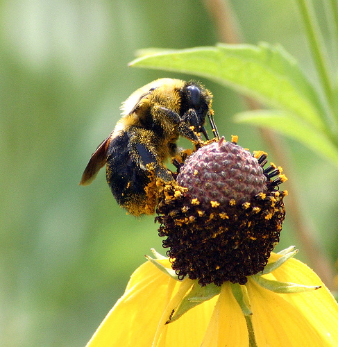
Train image
conv1 layer feature map
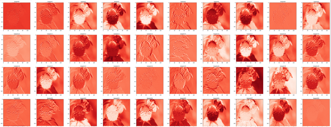
If you notice, the feature maps are flipped. The input images are horizontally flipped during augmentation. Similarly, you can visualize other layers of the network. In this project, I have visualized only the feature maps, as a next step, I want to cluster these features map vectors to find their behavior over the training phase.
Written on May 9th, 2021 by Karthik