Summary - Densenet

Densenet-Densely Connected Convolutional Networks Paper

Let’s understand Densenet.

In this paper, we embrace this observation and introduce the Dense Convolutional Network (DenseNet), which connects each layer to every other layer in a feed-forward fashion. Whereas traditional convolutional networks with L layers have L connections—one between each layer and its subsequent layer—our network has L(L+1) 2 direct connections. For each layer, the feature-maps of all preceding layers are used as inputs, and its own feature-maps are used as inputs into all subsequent layers.

In convolution neural network architectures we have seen networks stacked up with layers. In case of RESNET, there is a skip connection from one previous layer. In case of Densenet, there will be connections from all subsequent layers.

Crucially, in contrast to ResNets, we never combine features through summation before they are passed into a layer; instead, we combine features by concatenating them.

In RESNET, the skip connection are summed up with the present layer. The summation is an element wise operation, hence the shape of two elements should be same. The summation output will have same shape. Where as in DENSENET, the skip connections are concatenated.There is no constrain that both layers output should be of same shape for concatenating.

the l th layer has inputs, consisting of the feature-maps of all preceding convolutional blocks. Its own feature-maps are passed on to all L subsequent layers. This introduces L(L+1)/2 connections in an L-layer network, instead of just L, as in traditional architectures.

The total connections in the network is given by L(L+1)/2 . There are three dense block, each with 5 connections. Hence totally 15 connections.

Advantages of Densenet:

1. They alleviate the vanishing-gradient problem.
2. Strengthen feature propagation.
3. Encourage feature reuse.
4. Reduce the number of parameters.

What makes Densenet special ?

Instead of drawing representational power from extremely deep or wide architectures, DenseNets exploit the potential of the network through feature reuse, yielding condensed models that are easy to train and highly parameter efficient. Concatenating feature-maps learned by different layers increases variation in the input of subsequent layers and improves efficiency

Instead of carrying feature map information from deeper and wider previous layer networks.Densenet use feature reuse which reduces the number of parameters in the network. In the above image, the features learnt from Layer1 can be used by Layer 3. Hence Layer 3 doesn’t have to learn the same features. Layer 3 can directly access the features learnt by Layer 1 as they are concatenated.

Dense Block functions

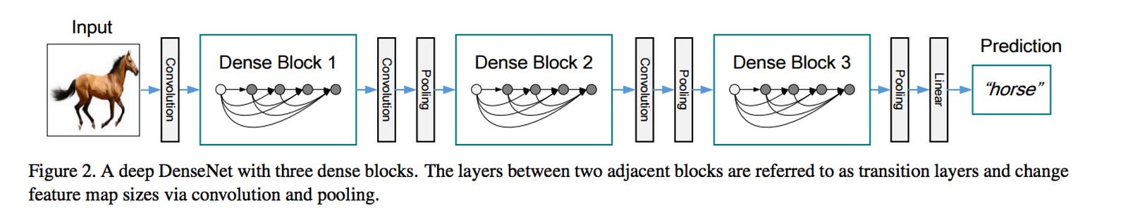
To further improve the information flow between layers we propose a different connectivity pattern: we introduce direct connections from any layer to all subsequent layers. Figure 1 illustrates the layout of the resulting DenseNet schematically. Consequently, the th layer receives the feature-maps of all preceding layers, x0, . . . , x−1, as input:

\(l^{th} \ layer \ receives \ the \ feature \ maps \ for \ all \ the \ preceding \ layers,\) `\(x_0,.........x_{l-1} \\ x_l = H_l ([x_0 , x_1,....x_{l-1}]) \ ( Eq \ 2)\)

where [x0, x1, . . . , x−1] refers to the concatenation of the feature-maps produced in layers 0, . . . , −1. Because of its dense connectivity we refer to this network architecture as Dense Convolutional Network (DenseNet). For ease of implementation, we concatenate the multiple inputs of `\(H_l{(·)}\) in eq. (2) into a single tensor.

Transition Block

Growth Rate

If each function H produces k feature maps, it follows that the `\(l_{th}\) layer has k0 + k ×(−1) input feature-maps, where k0 is the number of channels in the input layer. An important difference between DenseNet and existing network architectures is that DenseNet can have very narrow layers, e.g., k = 12. We refer to the hyperparameter k as the growth rate of the network.

Why we need Growth Rate ?

Each layer adds k feature-maps of its own to this state. The growth rate regulates how much new information each layer contributes to the global state. The global state, once written, can be accessed from everywhere within the network and, unlike in traditional network architectures, there is no need to replicate it from layer to layer.

Model compactness

To improve model compactness, we can reduce the number of feature-maps at transition layers. If a dense block contains m feature-maps, we let the following transition layer generate bθmc output featuremaps, where 0 <θ ≤1 is referred to as the compression factor. When θ = 1, the number of feature-maps across transition layers remains unchanged. We refer the DenseNet with θ <1 as DenseNet-C, and we set θ = 0.5 in our experiment. When both the bottleneck and transition layers with θ < 1 are used, we refer to our model as DenseNet-BC.

Implementation details

Before entering the first dense block, a convolution with 16 (or twice the growth rate for DenseNet-BC) output channels is performed on the input images. For convolutional layers with kernel size 3×3, each side of the inputs is zero-padded by one pixel to keep the feature-map size fixed. We use 1×1 convolution followed by 2×2 average pooling as transition layers between two contiguous dense blocks. At the end of the last dense block, a global average pooling is performed and then a softmax classifier is attached.

The feature-map sizes in the three dense blocks are 32× 32, 16×16, and 8×8, respectively. We experiment with the basic DenseNet structure with configurations {L = 40, k = 12}, {L = 100, k = 12} and {L = 100, k = 24}. For DenseNetBC, the networks with configurations {L = 100, k = 12}, {L= 250, k= 24} and {L= 190, k= 40} are evaluated.

Training on CIFAR-10

The two CIFAR datasets consist of colored natural images with 32×32 pixels. CIFAR-10 (C10) consists of images drawn from 10 and CIFAR-100 (C100) from 100 classes. The training and test sets contain 50,000 and 10,000 images respectively, and we hold out 5,000 training images as a validation set. We adopt a standard data augmentation scheme (mirroring/shifting) that is widely used for these two datasets. We denote this data augmentation scheme by a “+” mark at the end of the dataset name (e.g., C10+). For preprocessing, we normalize the data using the channel means and standard deviations. For the final run we use all 50,000 training images and report the final test error at the end of training.

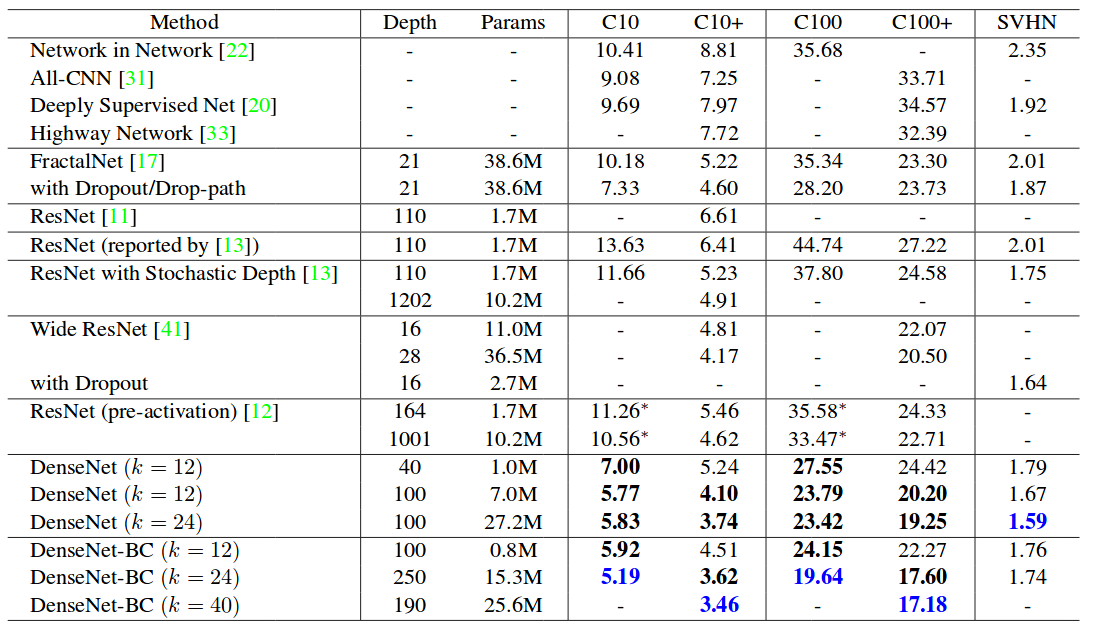
Training results from paper.

Written on October 25th, 2018 by Karthik