Siamese Network for duplicate detection

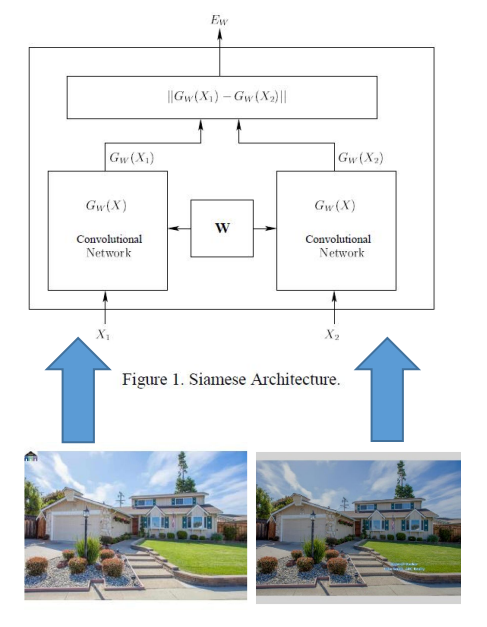
In this post, I will list out the application of Siamese network from the paper Using Siamese CNNs for Removing Duplicate Entries From Real-Estate Listing Databases.

Real estate databases are geo-specific. If a house to be put up for sale is located close to the geo boundary, a real estate listing agent will often list it in both databases. For example, a house located in Milpitas would often be listed in both East Bay and South Bay databases. The content of both database entries could be different to appeal to different demographics of each area.

Real estate brokerage firms do enter in cross-area sharing agreements and there are efforts underway to create a nation-wide sharing framework as well. Herein lies the problem: when data feeds from EastBay and SouthBay databases are aggregated, this results in two duplicate listings. The purpose of the project is to provide means to identify and flag these duplicates for future removal.

The challenging part ☹️

Contrary to what one might think, property’s street address by itself is not enough to identify the duplicate entries.

The good part 😍

Some of the most reliable indicators of duplicate listings are jpeg images uploaded by agents, but these can’t always be simply binary-compared since they may contain broker watermarks, be cropped, flipped or have post-processing visual effects such as color modifications.

Loss function and “difference” norm:

We tried both L1 and a square norm (L2) and found L2 to result in better accuracy and precision. Thus, in the end, we decided to use L2

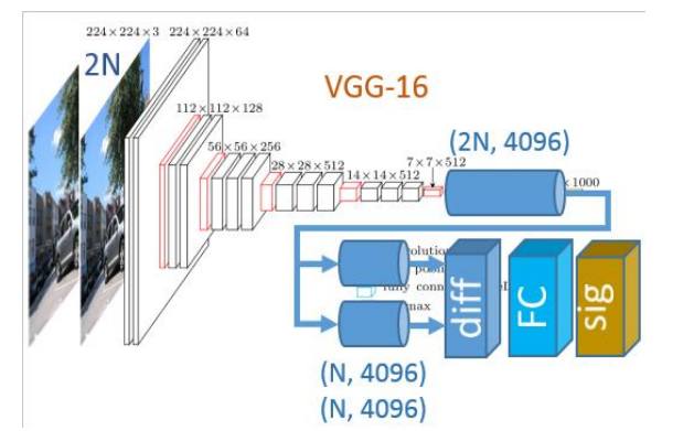
Activation function:

After experimenting with softmax cross-entropy function which seemed to be an over-kill for this 2-class logistics regression problem, we finally settled on using a sigmoid function.

Optimization:

We started with a plain SGD and were able to achieve accuracy on the order of 70%. We have also tried Adam optimization which took a while to get working in Tensorflow because it required initializing local variables, but found that it did not perform significantly better than traditional SGD, so we revered back to SGD and were able to achieve good results by lowering the learning rate and adjusting dropout which was used for the published results 🤩.

As expected, the majority of the time for this project was spent debugging TensorFlow code, preparing dataset, but mostly optimizing hyperparameters.

In particular, since we needed to deal with two different learning rates (one for training the newly-added layers and one for overall model training), we found ourselves spending three times as much effort on this task as we expected to.

🧠 Other challenging optimization task was experimenting with different image sizes, random flipping and cropping of training and validation images which was also affecting training accuracy.

Perhaps somewhat surprisingly, weight decay and dropout rate did not seem to significantly affect loss and accuracy values. Perhaps if we spent more time adjusting the learning rates, we would have reached a point where the effects of other hyperparameters became more pronounced.

Experiments/Results/Discussion:

As a primary success metric we used Accuracy which is defined as (TP+TN)/Total, where TP – “true positive” and TN – “true negative”.

For the test dataset, we also calculated Precision = TP/(TP + FP) and Recall = TP/(TP + FN)

Baseline:

Before embarking on building a convolutional neural network, we attempted a brute-force approach using a 1-Nearest Neighbor algorithm borrowed from CS231N assignment-1. We had to slightly modify our definition of the “labels” in order to make it work in the following way. Each image in our dataset of K images was assigned a label corresponding to its “similar” twin. Those without a twin, we assigned label ‘K+1’.

When training, we would first run our network with all VGG-16 weights “frozen” except for FC7 and the added FC_distance layer for several epoch (~5 epoch turned out to be sufficient as the loss function would stop improving afterwards). Then we would continue the run allowing all layers to be trained for 5-20 epochs, depending on the size of the training dataset

The nearest neighbor approach could cope to some extent with watermarking and color editing, it completely failed when images were flipped or significantly cropped. On a larger dataset, overall precision of Nearest Neighbor approach was found to be 24.4% which is in line with previous work on KNN algorithms.

We found the fact that the precision between different runs was 85-95%, indicating that there were very few false positives, i.e. the model would rarely mark two different test images as being the same (FP). It would, however, more often make a mistake of classifying two identical images as being different (FN), which is probably due to the fact that the images were cropped to 224x224 prior to being presented to the network.

Validation approach:

Since we enjoyed having access to a large dataset (far larger than we could process in a reasonable time on a single GPU available to us), we chose not to do K-fold validation, but instead drew data randomly from available dataset and for both training and validation.

Test data approach:

For testing holdout dataset, we selected a 50 images which we carefully reviewed to make sure they represented a reasonable approximation to real estate photo listings found in practice.

Test data analysis:

We carefully analyzed True Positives and False Positives responses of our network. We found that the network not only correctly recognized images on Fig 7 and 8 above (just like a Nearest-Neighbor network), but could also identify flipped image as being identical – something that the Nearest-Neighbor approach failed to do. Somewhat surprisingly, Siamese network consistently identified the two test images shown on Figure 10 as different, while Nearest Neighbor network did not have such difficulties.

Written on May 5th, 2022 by Karthik