Karthik Tech Blogs
Low dimension neural network training
Deep neural networks can be optimized in randomly-projected subspaces of much smaller dimensionality than their native parameter space. While such training is promising for more efficient and scalable optimization schemes, its practical application is limited by inferior optimization performance.
Here, we improve on recent random subspace approaches as follows:
-
Firstly, we show that keeping the random projection fixed throughout training is detrimental to optimization.
-
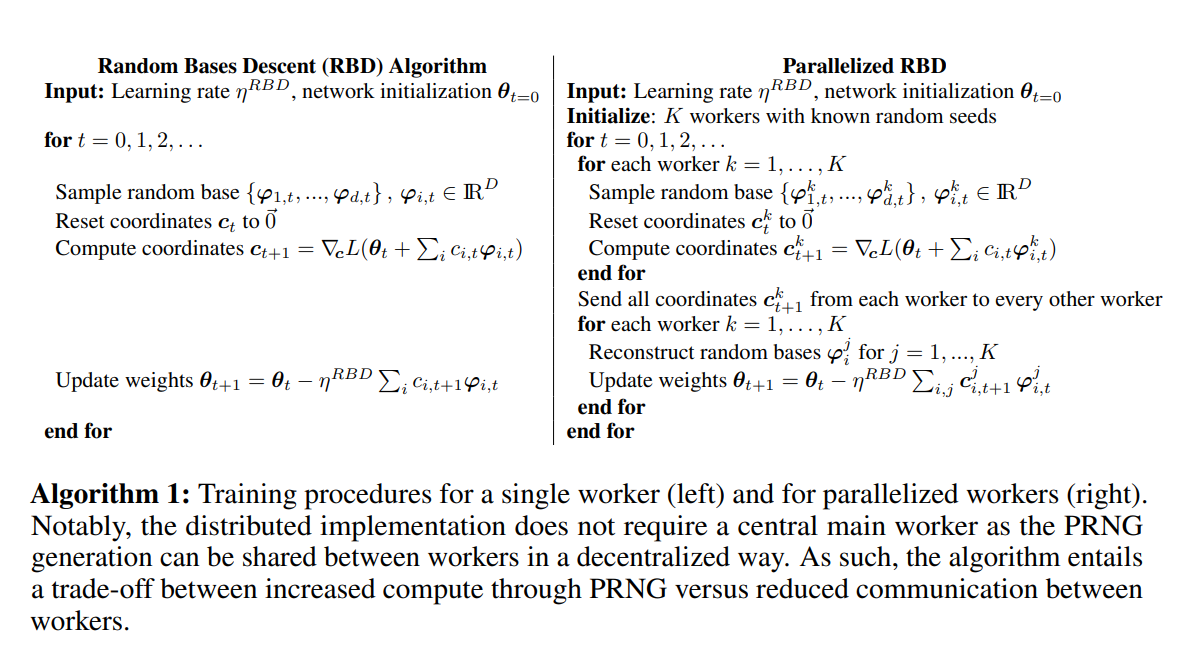
We propose re-drawing the random subspace at each step, which yields significantly better performance.
We realize further improvements by applying independent projections to different parts of the network, making the approximation more efficient as network dimensionality grows.
To implement these experiments, we leverage hardware-accelerated pseudo-random number generation to construct the random projections on-demand at every optimization step, allowing us to distribute the computation of independent random directions across multiple workers with shared random seeds.
This yields significant reductions in memory and is up to 10x faster for the workloads in question.
Empirical evidence suggests that not all of the gradient directions are required to sustain effective optimization and that the descent may happen in much smaller subspaces
Many methods are able to greatly reduce model redundancy while achieving high task performance at a lower computational cost
The paper observes that applying smaller independent random projections to different parts of the network and re-drawing them at every step significantly improves the obtained accuracy on fully-connected and several convolutional architectures
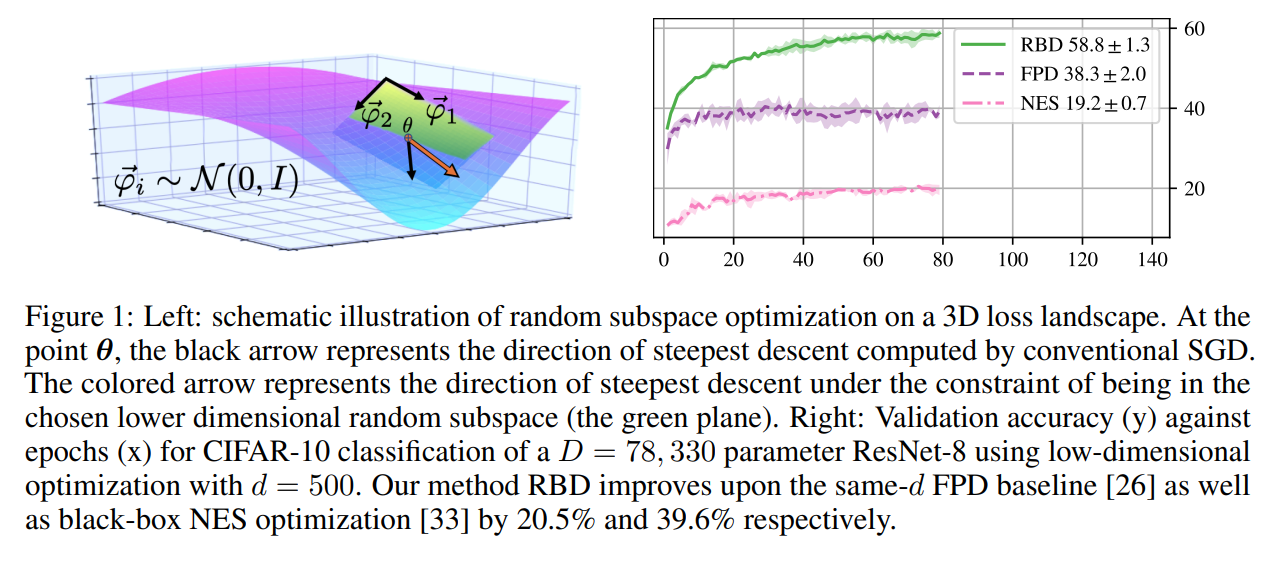
At the point θ, the black arrow represents the direction of steepest descent computed by conventional SGD. The colored arrow represents the direction of steepest descent under the constraint of being in the chosen lower dimensional random subspace (the green plane)
The below YouTube video will explain you about Basis, which is necessary to understand the further blog content.
To reduce the network training dimensionality, we seek to project into a lower dimensional random subspace by applying a D*d random projection matrix P to the parameters
If P’s column vectors are orthogonal and normalized, they form a randomly oriented base and
\(\\ c_t - \ can \ be \ interpreted \ as \ coordinates \ in \ the \ subspace.\)
As such, the construction can be used to train in a d-dimensional subspace of the network’s original D-dimensional parameter space.
In this formulation, however, any optimization progress is constrained to the particular subspace that is determined by the network initialization and the projection matrix.
To obtain a more general expression of subspace optimization, the random projection can instead be formulated as a constraint of the gradient descent in the original weight space.
The constraint requires the gradient to be expressed in the random base
\(\\ g^{(RB)}_t := \sum_{i=1}^{d} c_{i,t} * \varphi_{i,t}\)
with random basis vectors
\(\\ \{ \ \varphi_{i,t} \in \mathbb{R}^D \ \}_{i = 1}^{d}\)
and co-ordinates
\(\\ c_{i,t} \in \mathbb{R}\)
The gradient step
\[\\ g_t^{RB} \in \mathbb{R}^{D}\]can be directly used for descent in the native weight space following the standard update equation
\(\\ \theta_{t+1} := \theta_t - \eta_{RB} * g_t^{RB}\)
To obtain the d dimensional coordinate vector, we redefine the training objective itself to implement the random bases constraint
\(\\ L^{RBD}(c_1,.....,c_d) := L(\theta_t + \sum_{i=1}^{d} c_i * \varphi_{i,t})\)
Computing the gradient of this modified objective with respect to
\(\\ c = [c_1, ..., c_d]^T \ at \ c = \vec{0}\)
and substituting it back into the basis yields a descent gradient that is restricted to the specified set of basis vectors
\(\\ g_t^{RBD} := \sum_{i=1}^{d} \frac{\partial{L^{RBD}}}{\partial{c_i}}\)
This scheme never explicitly calculates a gradient with respect to θ, but performs the weight update using only the d> coordinate gradients in the respective base.
Conclusion:
- The paper introduced an optimization scheme that restricts gradient descent to a few random directions, re-drawn at every step.
- This provides further evidence that viable solutions of neural network loss landscape can be found, even if only a small fraction of directions in the weight space are explored.
- In addition, the paper shows that using compartmentalization to limit the dimensionality of the approximation can further improve task performance.