Karthik Tech Blogs
Optimization in Deep Learning
Paper: An overview of gradient descent optimization algorithms
This article will discuss about different optimization techniques that are widely employed in Neural Networks. This article focuses on optimizer selection strategy for desired Neural Networks.
Gradient Descent
Gradient descent is a way to minimize an objective function J(θ) parameterized by a model’s parameters θ ∈ R^d by updating the parameters in the opposite direction of the gradient of the objective function ∇_θ(J(θ)) w.r.t. to the parameters. The learning rate η determines the size of the steps we take to reach a (local) minimum.
Gradient descent variants
There are three variants of gradient descent, which differ in how much data we use to compute the gradient of the objective function. Depending on the amount of data, we make a trade-off between the accuracy of the parameter update and the time it takes to perform an update.
Batch gradient descent
As we need to calculate the gradients for the whole dataset to perform just one update, batch gradient descent can be very slow and is intractable for datasets that do not fit in memory. Batch gradient descent also does not allow us to update our model online, i.e. with new examples on-the-fly.
We then update our parameters in the direction of the gradients with the learning rate determining how big of an update we perform. Batch gradient descent is guaranteed to converge to the global minimum for convex error surfaces and to a local minimum for non-convex surfaces.
Stochastic gradient descent
Batch gradient descent performs redundant computations for large datasets, as it recomputes gradients for similar examples before each parameter update. SGD does away with this redundancy by performing one update at a time. It is therefore usually much faster and can also be used to learn online. SGD performs frequent updates with a high variance that cause the objective function to fluctuate heavily
While batch gradient descent converges to the minimum of the basin, the parameters are placed in, SGD’s fluctuation, on the one hand, enables it to jump to new and potentially better local minima. On the other hand, this ultimately complicates convergence to the exact minimum, as SGD will keep overshooting.
However, it has been shown that when we slowly decrease the learning rate, SGD shows the same convergence behaviour as batch gradient descent, almost certainly converging to a local or the global minimum for non-convex and convex optimization respectively.
Mini-batch gradient descent
Mini-batch gradient descent finally takes the best of both worlds and performs an update for every mini-batch of n training examples:
This way, it
- reduces the variance of the parameter updates, which can lead to more stable convergence;
- Can make use of highly optimized matrix optimizations common to state-of-the-art deep learning libraries that make computing the gradient w.r.t. a mini-batch very efficient.
Challenges
Vanilla mini-batch gradient descent, however, does not guarantee good convergence, but offers a few challenges that need to be addressed:
- Choosing a proper learning rate can be difficult.
- Learning rate schedules try to adjust the learning rate during training by e.g. annealing, i.e. reducing the learning rate according to a pre-defined schedule or when the change in objective between epochs falls below a threshold. These schedules and thresholds, however, have to be defined in advance and are thus unable to adapt to a dataset’s characteristics.
- The same learning rate applies to all parameter updates. If our data is sparse and our features have very different frequencies, we might not want to update all of them to the same extent, but perform a larger update for rarely occurring features.
- Another key challenge of minimizing highly non-convex error functions common for neural networks is avoiding getting trapped in their numerous suboptimal local minima. Dauphin et al argue that the difficulty arises in fact not from local minima but from saddle points, i.e. points where one dimension slopes up and another slopes down. These saddle points are usually surrounded by a plateau of the same error, which makes it notoriously hard for SGD to escape, as the gradient is close to zero in all dimensions.
Gradient descent optimization algorithms
Momentum
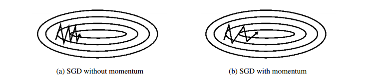
Momentum is a method that helps accelerate SGD in the relevant direction and dampens oscillations. It does this by adding a fraction γ (gamma) of the update vector of the past time step to the current update vector.
The momentum term increases for dimensions whose gradients point in the same directions and reduces updates for dimensions whose gradients change directions. As a result, we gain faster convergence and reduced oscillation
Nesterov accelerated gradient
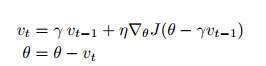
Nesterov accelerated gradient (NAG) is a way to give our momentum term this kind of prescience. Computing θ− γ.v_(t−1) thus gives us an approximation of the next position of the parameters (the gradient is missing for the full update), a rough idea where our parameters are going to be. We can now effectively look ahead by calculating the gradient not w.r.t. to our current parameters θ but w.r.t. the approximate future position of our parameters:
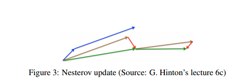
Again, we set the momentum term γ to a value of around 0.9. While Momentum first computes the current gradient (small blue vector in Figure 3) and then takes a big jump in the direction of the updated accumulated gradient (big blue vector), NAG first makes a big jump in the direction of the previous accumulated gradient (brown vector), measures the gradient and then makes a correction (green vector). This anticipatory update prevents us from going too fast and results in increased responsiveness, which has significantly increased the performance of RNNs on a number of tasks
Now that we are able to adapt our updates to the slope of our error function and speed up SGD in turn, we would also like to adapt our updates to each individual parameter to perform larger or smaller updates depending on their importance.
Adagrad
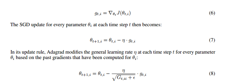
It adapts the learning rate to the parameters, performing larger updates for infrequent and smaller updates for frequent parameters. For this reason, it is well-suited for dealing with sparse data.
we performed an update for all parameters θ at once as every parameter θi used the same learning rate η. As Adagrad uses a different learning rate for every parameter θ_i at every time step t, we first show Adagrad’s per-parameter update, which we then vectorize.
One of Adagrad’s main benefits is that it eliminates the need to manually tune the learning rate. Most implementations use a default value of 0.01 and leave it at that.
Adagrad’s main weakness is its accumulation of the squared gradients in the denominator: Since every added term is positive, the accumulated sum keeps growing during training. This in turn causes the learning rate to shrink and eventually become infinitesimally small, at which point the algorithm is no longer able to acquire additional knowledge.
Adadelta
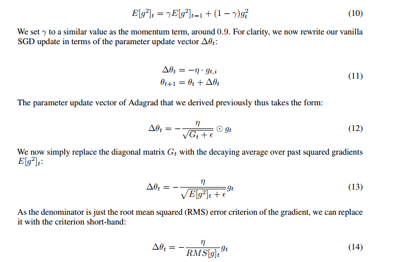
Adadelta is an extension of Adagrad that seeks to reduce its aggressive, monotonically decreasing learning rate. Instead of accumulating all past squared gradients, Adadelta restricts the window of accumulated past gradients to some fixed size w. Instead of inefficiently storing w previous squared gradients, the sum of gradients is recursively defined as a decaying average of all past squared gradients. The running average at time step t then depends (as a fraction γ similarly to the Momentum term) only on the previous average and the current gradient.
With Adadelta, we do not even need to set a default learning rate, as it has been eliminated from the update rule.
RMSprop
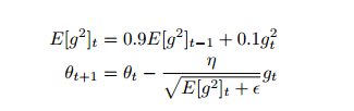
RMSprop and Adadelta have both been developed independently around the same time stemming from the need to resolve Adagrad’s radically diminishing learning rates.
RMSprop as well divides the learning rate by an exponentially decaying average of squared gradients.
Hinton suggests γ to be set to 0.9, while a good default value for the learning rate η is 0.001
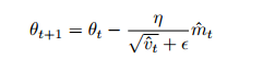
Adam
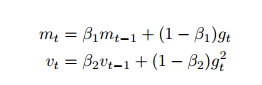
Adam also keeps an exponentially decaying average of past gradients m_t, similar to momentum.
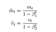
m_t and v_t are estimates of the first moment (the mean) and the second moment (the uncentered variance) of the gradients respectively, hence the name of the method. As m_t and v_t are initialized as vectors of 0’s, the authors of Adam observe that they are biased towards zero, especially during the initial time steps, and especially when the decay rates are small (i.e. β1 and β2 are close to 1).
They counteract these biases by computing bias-corrected first and second moment estimates.
They show empirically that Adam works well in practice and compares favorably to other adaptive learning-method algorithms.
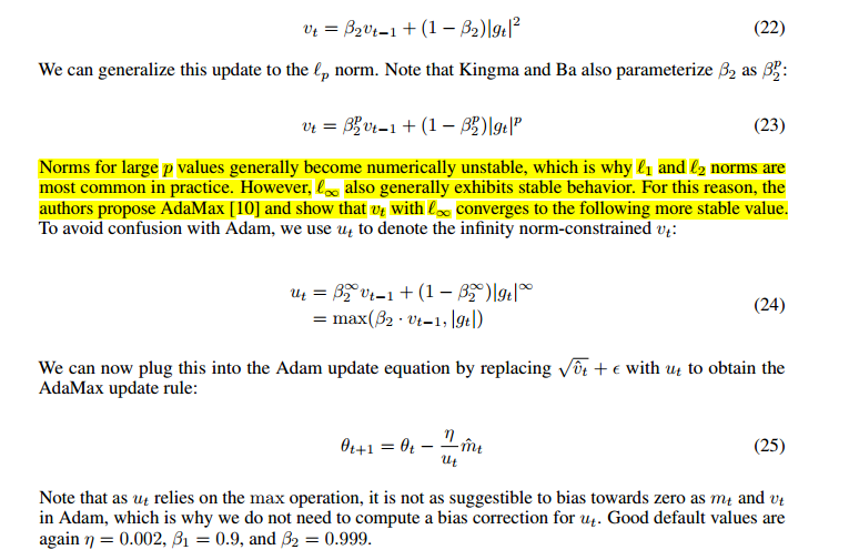
AdaMax
The v_t factor in the Adam update rule scales the gradient inversely proportionally to the `2 norm of the past gradients (via the v_(t−1) term) and current gradient.
Nadam
RMSprop contributes the exponentially decaying average of past squared gradients v_t, while momentum accounts for the exponentially decaying average of past gradients m_t. We have also seen that Nesterov accelerated gradient (NAG) is superior to vanilla momentum. Nadam (Nesterov-accelerated Adaptive Moment Estimation) thus combines Adam and NAG. In order to incorporate NAG into Adam, we need to modify its momentum term m_t.
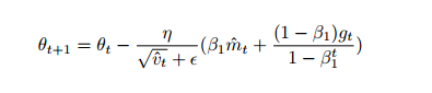
Notice that rather than utilizing the previous momentum vector m_(t−1), we now use the current momentum vector m_t to look ahead. In order to add Nesterov momentum to Adam, we can thus similarly replace the previous momentum vector with the current momentum vector
Which optimizer to use?
If your input data is sparse, then you likely achieve the best results using one of the adaptive learning-rate methods. An additional benefit is that you will not need to tune the learning rate but will likely achieve the best results with the default value.
Adam, finally, adds bias-correction and momentum to RMSprop. Insofar, RMSprop, Adadelta, and Adam are very similar algorithms that do well in similar circumstances. Kingma et al show that its bias-correction helps Adam slightly outperform RMSprop towards the end of optimization as gradients become sparser. Insofar, Adam might be the best overall choice.
Interestingly, many recent papers use vanilla SGD without momentum and a simple learning rate annealing schedule. As has been shown, SGD usually achieves to find a minimum, but it might take significantly longer than with some of the optimizers, is much more reliant on a robust initialization and annealing schedule, and may get stuck in saddle points rather than local minima. Consequently, if you care about fast convergence and train a deep or complex neural network, you should choose one of the adaptive learning rate methods.
Parallelizing and distributing SGD
Given the ubiquity of large-scale data solutions and the availability of low-commodity clusters, distributing SGD to speed it up further is an obvious choice. SGD by itself is inherently sequential: Step-by-step, we progress further towards the minimum. Running it provides good convergence but can be slow particularly on large datasets. In contrast, running SGD asynchronously is faster, but suboptimal communication between workers can lead to poor convergence. Additionally, we can also parallelize SGD on one machine without the need for a large computing cluster
Hogwild!
They show that in this case, the update scheme achieves almost an optimal rate of convergence, as it is unlikely that processors will overwrite useful information.
Downpour SGD
Downpour SGD is an asynchronous variant of SGD. It runs multiple replicas of a model in parallel on subsets of the training data. These models send their updates to a parameter server, which is split across many machines. Each machine is responsible for storing and updating a fraction of the model’s parameters. However, as replicas don’t communicate with each other e.g. by sharing weights or updates, their parameters are continuously at risk of diverging, hindering convergence.
Delay-tolerant Algorithms for SGD
McMahan and Streeter extend AdaGrad to the parallel setting by developing delay-tolerant algorithms that not only adapt to past gradients, but also to the update delays. This has been shown to work well in practice.
Elastic Averaging SGD
Elastic Averaging SGD (EASGD), which links the parameters of the workers of asynchronous SGD with an elastic force, i.e. a center variable stored by the parameter server. This allows the local variables to fluctuate further from the center variable, which in theory allows for more exploration of the parameter space. They show empirically that this increased capacity for exploration leads to improved performance by finding new local optima.
Additional strategies for optimizing SGD
Shuffling and Curriculum Learning
Generally, we want to avoid providing the training examples in a meaningful order to our model as this may bias the optimization algorithm. Consequently, it is often a good idea to shuffle the training data after every epoch. On the other hand, for some cases where we aim to solve progressively harder problems, supplying the training examples in a meaningful order may actually lead to improved performance and better convergence. The method for establishing this meaningful order is called Curriculum Learning.
Batch normalization
To facilitate learning, we typically normalize the initial values of our parameters by initializing them with zero mean and unit variance. As training progresses and we update parameters to different extents, we lose this normalization, which slows down training and amplifies changes as the network becomes deeper.
Batch normalization reestablishes these normalizations for every mini-batch and changes are back- propagated through the operation as well. By making normalization part of the model architecture, we are able to use higher learning rates and pay less attention to the initialization parameters. Batch normalization additionally acts as a regularizer, reducing (and sometimes even eliminating) the need for Dropout.
Gradient noise
Neelakantan et al. added noise that follows a Gaussian distribution to each gradient update.
They show that adding this noise makes networks more robust to poor initialization and helps training particularly deep and complex networks. They suspect that the added noise gives the model more chances to escape and find new local minima, which are more frequent for deeper models.