A generative model G that captures the data distribution. A discriminative model D estimates the probability that a sample came from the training data rather than G.
Dis_probability = ( Number of samples from training data)/( Total Number of Samples generated by generator)
The training procedure for Generator is to maximize the probability of Discriminator making a mistake. This way the Generator generates samples from the training distribution and when the discriminator fails to detect that, then the discriminator loss increases forcing it improving the accuracy. Generator and Discriminator are multi layer perceptrons where the entire network can be trained with backpropagation.
In the proposed adversarial nets framework, the generative model is pitted against an adversary: a discriminative model that learns to determine whether a sample is from the model distribution or the data distribution.
We can train both models using only the highly successful backpropagation and dropout algorithms and sample from the generative model using only forward propagation.
Adversarial nets:
To learn the generator’s distribution p_g over data x, we define a prior on input noise variables p_z(z), then represent a mapping to data space as G(z; θ_g), where G is a differentiable function represented by a multilayer perceptron with parameters θ_g
A second multilayer perceptron D(x; θ_d) that outputs a single scalar.
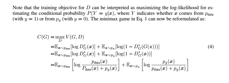
D(x) represents the probability that x came from the data rather than p_g
We train D to maximize the probability of assigning the correct label to both training examples and samples from G
We simultaneously train G to minimize log(1 − D(G(z)))
In practice, we must implement the game using an iterative, numerical approach. Optimizing D to completion in the inner loop of training is computationally prohibitive, and on finite datasets would result in overfitting.
Instead, we alternate between k steps of optimizing D and one step of optimizing G.
This results in D being maintained near its optimal solution, so long as G changes slowly enough.
Early in learning, when G is poor, D can reject samples with high confidence because they are clearly different from the training data.
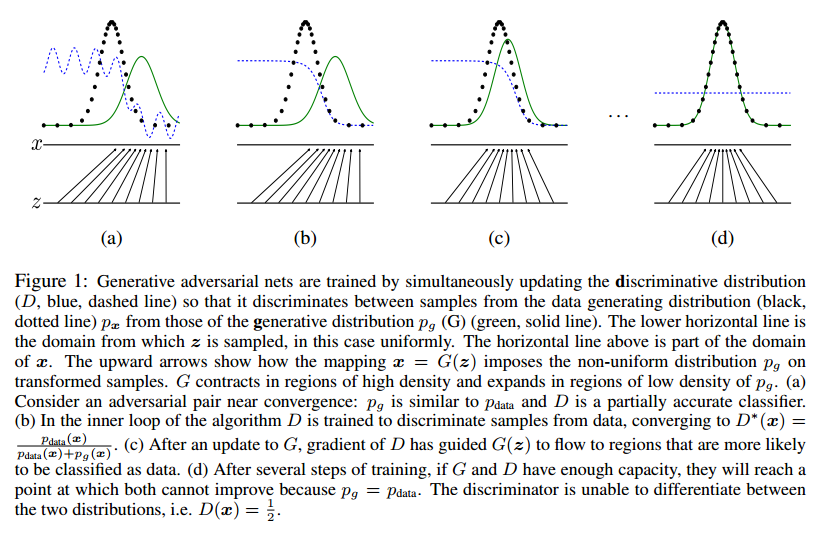
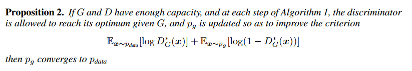
The generator G implicitly defines a probability distribution p_g as the distribution of the samples G(z) obtained when z ∼ p_z. Therefore, we would like Algorithm 1 to converge to a good estimator of p_data, if given enough capacity and training time.
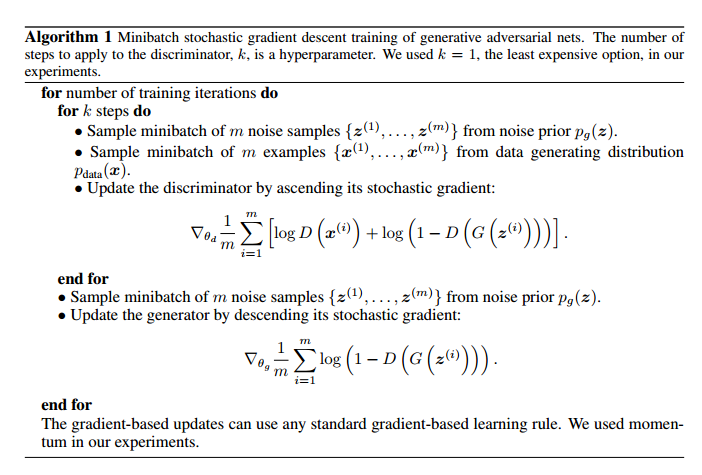
- The number of training iterations can be viewed as Epochs.
- K steps training for discriminator for every step training for generator.
- Sample minibatch m noise samples from noise prior.
- Sample minibatch m examples from data generating distribution.
- Update the discriminator by ascending its stochastic gradient.
- D(x^(i)) gives the probability of data belonging to training distribution.
- D(G(z^(i))) gives the probability of data belonging to Generative distribution.
- Sample minibatch m noise samples from noise prior for generator.
- Update the generator by descending its stochastic gradient.
- The stochastic gradient is calculated on D(G(z^(i))).
The gradient-based updates can use any standard gradient-based learning rule. We used momentum in our experiments.
Global Optimality of p_g = p_data.
There are two possibility of Discriminator during training.
- Discriminator predicts generator image as a sample from training data distribution. In this case, the prediction probability is 1. The discriminator is been fooled by the generator’s output.
- Discriminator predicts generator image is not a sample from training data distribution. In this case, the prediction probability is 0. The discriminator couldn’t be fooled by the generator’s output since the generator output quality is bad.
Convergence of Algorithm 1
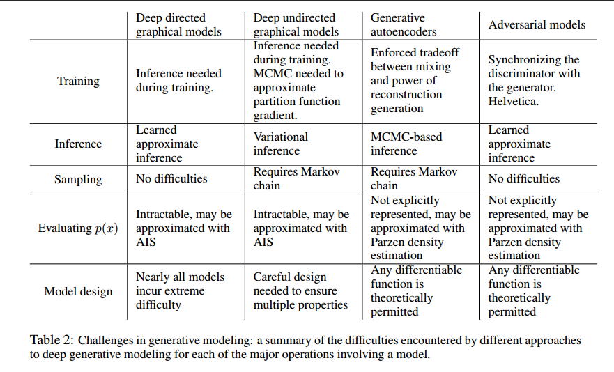
Challenges in Generative modelling
Challenges in training GANs
-
Vanishing Gradients
If the discriminator is good at predicting fake and real images, then it gets complicated to fool the discriminator network. This hinders generator training which causes vanishing gradient problem.
- Wasserstein loss is designed to prevent vanishing gradient problem even when the discriminator is trained to optimality.
Good discriminator > Low Prediction Error > "Generated image is not coming from training distribution" > Low loss ( Causes Vanishing Gradient Problem )
Bad discriminator > High Prediction Error > "Generated image is coming from training distribution" > High loss
-
Model Collapse
A scenario where the generator is trained to generate the same single image and the discriminator keeps on predicting on the same single image that it is a part of training distribution.
- Wasserstein loss prevents generator network getting stabilised with same single output. This motivates the generator network to try something new.
- Unrolled GANs use a generator loss function that incorporates not only the current discriminator’s classifications, but also the outputs of future discriminator versions. Hence the generator cannot optimize for single version of the discriminator.
-
Convergence Failure
It is complicated to obtain Nash equilibrium.
- Adding noise to discriminator input.
- Penalizing discriminator weights.
Different types of GANs
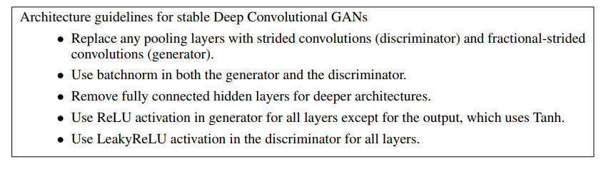
DCGAN - Deep Convolution Generative Adversarial Networks
- A set of contraints is introduced on the architectural topology of Convolutional GANs.
- Deep convolutional adversarial pair learns a hierarchy of representations from object parts to scenes in both the generator and discriminator.
- A trained discriminator is employed for image classification providing competitive performance with other unsupervised algorithms.
Three important changes is done on the generator network:
-
Replacement of maxpooling with strided convolution. This approach in our generator, allowing it to learn its own spatial upsampling, and discriminator.
-
The fully connected layers is been replaced with global average pooling. The outcome of using global average pooling increased model stability but hurt convergence speed.
-
Batch normalization which stabilizes learning by normalizing the input to each unit to have zero mean and unit variance. This helps with training problems such as poor initialization and helps in gradient flow in deeper networks.
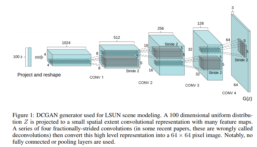
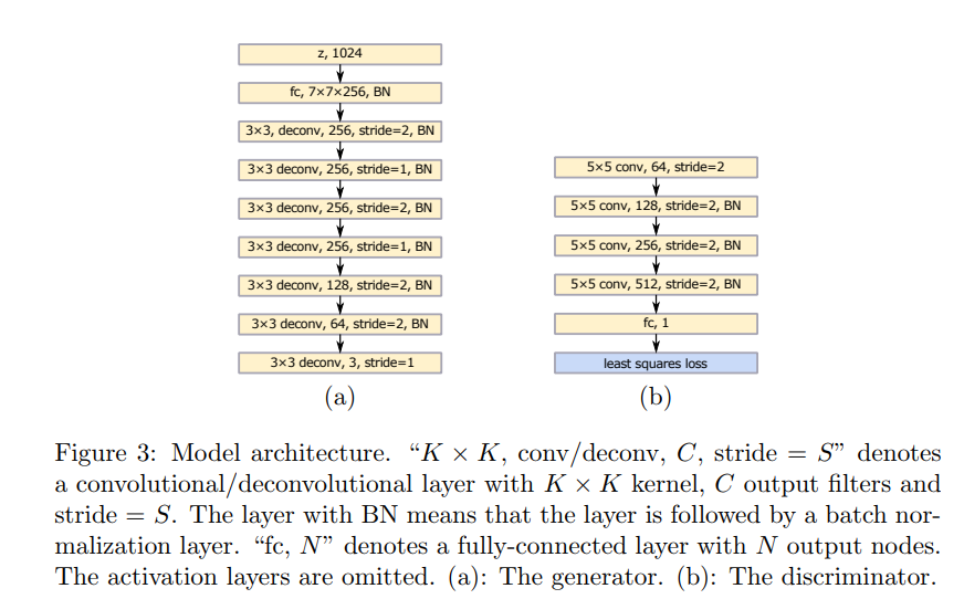
Generator Architecture:
CGAN - Conditional Generative Advesarial Networks
This is a conditional version of GANs, which can be constructed by feeding additional data through which we wish to condition the output on both the generator and the discriminator.
This additional data can be label information or output from other modalities.
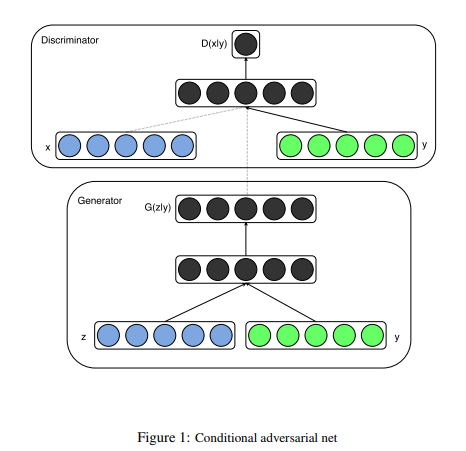
The green block vector is the additional condition data (y). y is combined in joint hidden representation and the adversarial training framework allows for considerable flexibility in how this hidden representation is composed.
In the discriminator x and y are presented as inputs and to a discriminative function.
LSGAN - Least Square GAN
Regular GANs hypothesize the discriminator as a classifier with the sigmoid cross entropy loss function. However, that this loss function may lead to the vanishing gradients problem during the learning process. To overcome such a problem, in this paper the Least Squares Generative Adversarial Networks was proposed.
InfoGan - Interpretable Representation Learning by Information Maximizing GAN
An information-theoretic extension to the Generative Adversarial Network that is able to learn disentangled representations in a completely unsupervised manner.
InfoGAN is a generative adversarial network that also maximizes the mutual information between a small subset of the latent variables and the observation.
Specifically, InfoGAN successfully disentangles writing styles from digit shapes on the MNIST dataset, pose from lighting of 3D rendered images, and background digits from the central digit on the SVHN dataset. It also discovers visual concepts that include hair styles, presence/absence of eyeglasses, and emotions on the CelebA face dataset.
In this paper, single unstructured noise vector has been decomposed into two parts:
- z, which is treated as source of incompressible noise.
- c, which we will call the latent code and will target the salient structured semantic features of the data distribution.
GANs Podcast
An intuitive conversation about GANs with Lex Fridman and Ian Goodfellow.